Authors: Bahar Biller and Jagdishwar Mankala
Inspired by a real-world project at a major aircraft manufacturer, this post explores how incorporating operational variables can improve asset survival predictions. Operational variables that can account for variability in time-to-failure include speed, vibration, and ambient temperature. By using a synthetically generated data set, we present examples of these explanatory variables, demonstrate how to integrate them into statistical models by using PROC PHREG, and highlight the significance of considering operational variables for accurate asset lifetime prediction.
Describing the use case
In this post, we revisit a scenario from Asset Performance Management with SAS: Improving Asset Uptimes while Reducing Cost. Now, we add the challenge of incorporating operational variables related to the settings and environmental conditions to which the asset is exposed. Consider the scenario where we remove an asset for inspection and testing. We then send it to the repair shop and record the times between asset removals in a historical data set.
Based on the inspection results at the repair shop, we determine whether the asset has failed. If the asset fails, we either repair or replace it. So, the removal event is marked as failure = 1. If the asset is found to be in good condition and does not require repair or replacement, the removal event is marked as failure = 0. Thus, the data set includes right-censored data represented by the variable failure.
Our earlier post describes fitting a Weibull distribution function to the right-censored data set by using PROC LIFEREG. Then, we assessed the model fit by using PROC LIFETEST. In this post, we assume the data set includes not only the times between removals but also the asset’s journey. That is, tracking its operational settings and environmental conditions.
Consequently, multiple events are observed between consecutive removals, with the values of operational variables such as speed and vibration, and environmental conditions like ambient temperature, changing over time. We demonstrate how PROC PHREG can leverage this additional data layer to quantify its impact on the instantaneous risk of failure at a particular time point. This approach enhances the accuracy of asset survival function predictions, given that the asset has survived up to that time.
Introducing the historical data set
Table 1 shows the first ten entries from a synthetically generated data set of 5000 rows. These are named ops_data and detail the time-to-removal for an asset. The first column, removal_id, indexes the removal events. Although the table displays only two removal events (removal_id = 1 and removal_id = 2), the entire data set contains 1000 removal events. The value in the stop column of the last row associated with a removal_id indicates the number of hours between asset removals. The columns ops_tmp, ops_spd, and ops_vib represent the cumulative hours the asset has operated in high-temperature, high-speed, and high-vibration zones. These are the operational variables (covariates) that might affect the asset’s failure rate. Their values monotonically increase for each removal_id.
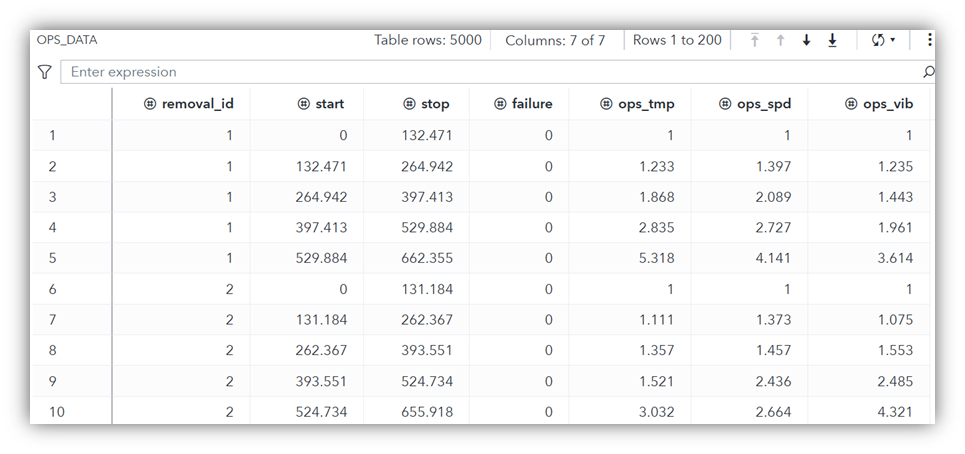
To illustrate the historical data set, we chose three operational variables. However, there is no restriction on the total number of operational variables that can be investigated. For every removal_id, Table 1 shows five consecutive time periods of equal length. Start and stop indicate the hours at which a period starts and ends. When moving from one period to the next, at least one operational variable changes. For simplicity, we assumed five equal-length periods.
However, the length of a period (stop–start) and the total number of periods until the removal can vary. The only requirement is that at least one operational variable changes with each period for each removal_id. We refer to this as having inputs in the counting process style. If a historical data set lacks this style, we need to preprocess the data.
Finally, the failure column value in the last row associated with a specific removal_id is either 0 or 1. This indicates whether the asset has failed. For other rows, the value of failure must be 0. Consequently, the historical data set includes the following primary columns: removal_id, start, stop, failure, and the cumulative values of all operational variables, used by PROC PHREG for reliability modeling. Keeping only the last row of each removal_id provides the event data illustrated in our previous blog without the operational variables. Finally, we split the data set into training and test sets with an 80:20 split ratio, naming them train_ops_data and test_ops_data.
Modeling reliability
Our objectives are twofold. One is to identify operational variables that significantly affect the asset failure rate. The other is to quantify these impacts. The historical data contains multiple events per removal, and the operational variables are time-dependent. These challenges are overcome by performing regression modeling with PROC PHREG using the counting process style. This procedure fits the Cox proportional hazards model. Also, it provides a p-value for each operational variable to determine its statistical significance. It estimates hazard ratios to quantify the impact on the asset’s failure rate as well.
Recall that the cumulative distribution function, F(t), describes the probability of an asset’s lifetime being less than or equal to time t. A simple transformation of this function produces the survival function S(t), where S(t) = 1-F(t). The survival function describes the probability that the asset survives past time t.
The Cox proportional hazards model, on the other hand, focuses on the hazard rate h(t), defined by [dF(t)/dt]/S(t), characterizing the instantaneous rate of failure at time t. It also expresses h(t) as h\(_0\)(t) exp(x\(\beta_x)\), where x represents the covariates, \(\beta_x\) their regression coefficients, x\(\beta_x\) the risk score, and h\(_0\)(t) the baseline hazard rate obtained for x=0. Thus, the hazard ratio associated with a covariate is the exponential function of its regression coefficient.
Figure 1 shows the code snippet for Cox regression modeling with PROC PHREG, including the operational variables ops_spd, ops_vib, and ops_tmp. The data statement specifies the training data set train_ops_data, while the model statement defines the survival model, including these variables. The model output identifies the cumulative hours spent in high-speed and high-vibration zones (ops_spd and ops_vib) as statistically significant, with p-values of 0.0024 and 0.0003, respectively.
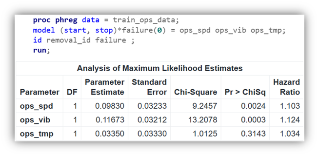
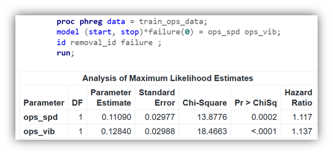
Figure 2 repeats the model fitting by using only these two variables. This shows that the asset failure rate increases by 11.7% (hazard ratio 1.117) for each additional hour spent in the high-speed zone. And increases by 13.7% (hazard ratio 1.137) for each additional hour spent in the high-vibration zone.
Predicting survival probabilities
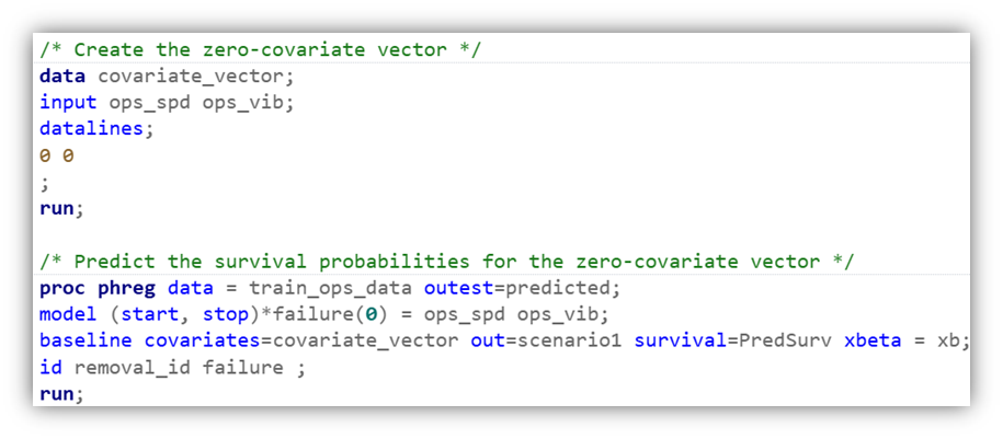
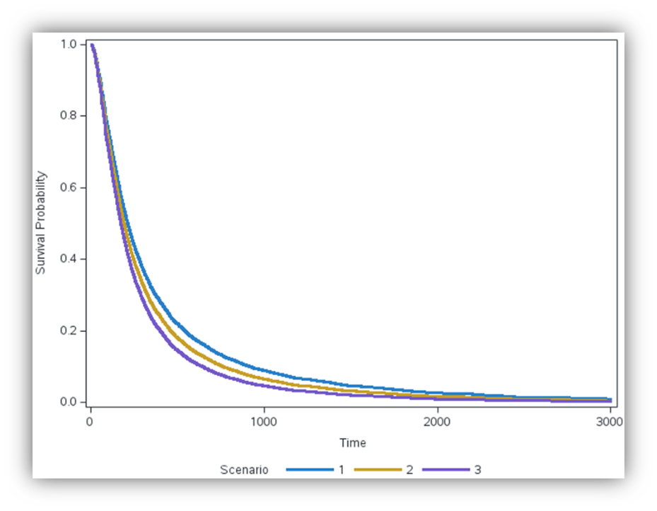
Now, we describe how to generate survival curves for different values of operational variables by using the baseline statement in PROC PHREG. We use the DATA step to create three vectors of (ops_spd, ops_vib): (0,0), (0.5,0.5), and (1,1), referred to as Scenario 1, Scenario 2, and Scenario 3. Applying PROC PHREG with the baseline statement to these vectors, we predict survival probabilities for the specified values of the operational variables. Figure 3 shows how to do this for the first scenario. Figure 4 illustrates the survival curves resulting from all three scenarios.
The comparison of the survival curves shows that survival probability decreases with more time spent in high-speed and high-vibration zones. For example, if the asset has not been operated in any high-speed and high-vibration zones (Scenario 1), the probability of surviving beyond 1000 hours is 9%. However, if the asset has been operated for half an hour in each zone (Scenario 2), the probability of surviving beyond 1000 hours decreases to 7%. Finally, if the asset operates for an hour in each zone (Scenario 3), the survival probability reduces to 5%. These observations align with the impact of these operational variables on the asset failure rate, as quantified in Figure 2.
Assessing the model
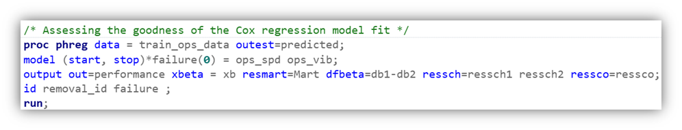
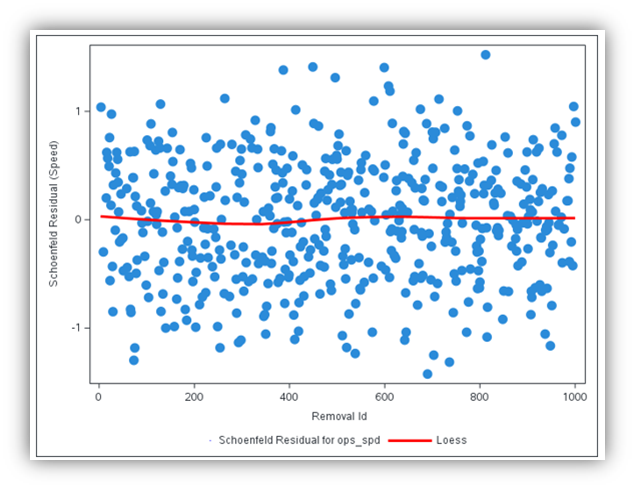
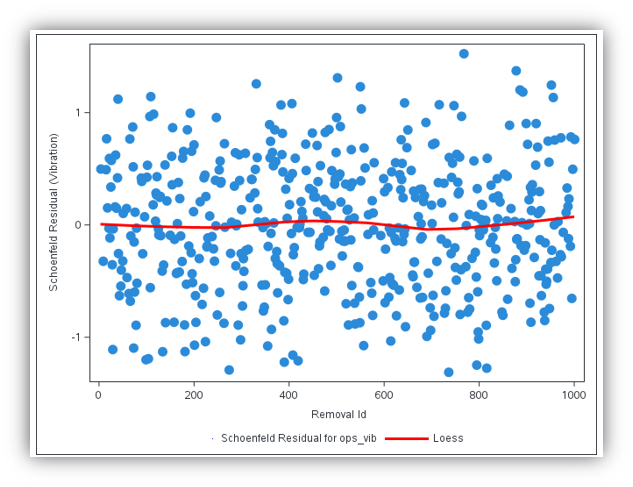
By using the output statement in PROC PHREG produces data sets with predicted values and performance statistics, such as risk score (xbeta), influence statistics (dfbeta), and various residuals (resmart for Martingale residuals, ressch for Schoenfeld residuals, ressco for score residuals). Figure 5 shows the code snippet with the output statement. Figures 6, 7, and 8 provide three visualizations from the performance output data set.
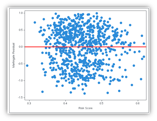
Plotting risk score on the x-axis and Martingale residuals on the y-axis (Figure 6) shows a random scatter around zero, indicating a good model fit. The graph of Schoenfeld residuals against removal_id for each operational variable (Figures 7 and 8) presents loess curves that are flat and close to zero, suggesting the proportional hazard model assumption holds and Cox regression is a suitable modeling approach to understanding the impact of operational variables on the asset failure rate.
Finally, we use the performance output data set to obtain an average risk quantification by applying the exponential function to the risk score (xbeta=xb) and multiplying exp(xb) by the difference of the start and stop columns for each row. We compute the resulting statistic \(\sum((stop-start)*exp(xb)/\sum(stop-start)\) as 1.599 for the training data set and 1.608 for the test data set. We estimate the survival functions of the training and test data sets by multiplying the exponential functions of these statistics with the baseline survival probabilities recorded in the scenario1 output data set (Figure 3). In addition, we find that the survival function from the test data set is very close to that from the training data set.
To conclude, PROC PHREG is a suitable choice for modeling our time-to-removal data set. This tracks changes in environmental conditions and operational settings over time. The goodness of the fitted model is investigated by using the output statement, as shown in Figure 5. The analysis of the maximum likelihood estimates in Figure 2 identifies the cumulative hours spent in high-speed and high-vibration zones as the operational variables with a statistically significant impact on the asset’s failure rate. It further quantifies this impact through the hazard ratios 1.117 and 1.137, indicating that high-speed zone hours increase the asset failure rate by 11.7% and high-vibration zone hours by 13.7%. Finally, it computes the probability of the asset surviving beyond a given duration, based on specific operational conditions. As illustrated in Figure 4, this highlights the importance of operational variables in enhancing asset lifetime predictions.
Summary
This post explains how to incorporate operational variables, or covariates, into predicting asset survival probabilities. The dynamic nature of these covariates and tracking the asset’s history until the next removal complicate predicting the asset’s lifetime under varying operational conditions. By using the PROC PHREG procedure, we can effectively address these challenges. This provides the historical data set that follows the counting process style and enhances asset lifetime prediction by integrating operational variables into the statistical modeling. The ability of SAS to handle censored data and perform advanced statistical analyses makes it an invaluable tool for asset performance management. Leveraging these capabilities improves predictions of asset lifetimes, ultimately leading to better decision-making and enhanced asset performance management.
Author Jagdishwar Mankala
Senior Data Scientist, SAS Pune Applied AI and Modeling
Jagdishwar Mankala is a Senior Data Scientist in the SAS Pune Applied AI and Modeling Division. He has over three years of experience specializing in optimization models, including inventory optimization and retail allocation. He holds a Master of Technology in Manufacturing Engineering from the Indian Institute of Technology (IIT) Bombay. Jagdishwar is passionate about leveraging data-driven insights to solve real-world challenges. Outside of work, he enjoys playing cricket, table tennis, and pencil sketching.