Asset Performance Management with SAS: Improving Asset Uptimes while Reducing Cost

An effective preventive maintenance practice maximizes asset uptime while minimizing the need to hold large amounts of spare parts inventory. Development of such a practice requires advanced analytics capability to accurately predict asset lifetime distributions in the presence of right-censored data sets. Motivated by a real project at a large aircraft manufacturer, this post will address asset lifetime prediction considering an asset with a synthetically generated historical data set. It will describe a solution built on SAS reliability modeling with the LIFEREG and LIFETEST procedures.

Use case description

Consider a scenario where a machine part, referred to as an asset, is removed and sent to the repair shop. Each removal is tracked with a variable named removal_id. An event data set records the number of hours between part removals. Let’s call the corresponding column of this data set time_to_removal. At the repair shop, it is determined whether the part has really failed. If it is found that the part has not failed, then the part is routed to the warehouse inventory of its supply chain network. This outcome is recorded as failure = 0 in the event data set. If it is found that the part has failed, then it is scrapped, and a procurement order is placed. This outcome is recorded as failure = 1. Consequently, the event data contains three primary columns: removal_id, time_to_removal, and failure. Because the failure column would be composed of 0s and 1s, the historical event data are right-censored. Unfortunately, this complicates the prediction of the asset lifetime distribution. To help our customers develop effective preventive maintenance policies, it is important to equip them with the capability to accurately predict the lifetimes of their assets despite the censored nature of the data set on hand. The question we ask in this post is how SAS could provide our customers such analytical capability. We answer this question in three main steps, demonstrated in Figure 1. We first discuss synthetic event data generation. Then, we perform Weibull regression modeling. Finally, we describe how to assess the performance of the resulting reliability model.

Figure 1: Three steps of asset lifetime prediction - asset performance management — Figure 1: Three steps of asset lifetime prediction

Synthetic data generation

First, we create an example event data set by using a SAS DATA step. We synthetically generate 1000 rows of numerical values for removal_id, time_to_removal, and failure and name the resulting data set event_data.sas7bdat. We set the censoring percentage to 35%; i.e., the number of rows with failure = 0 is expected to be 350. Figure 2 illustrates the first 15 rows of the resulting data set together with a histogram of the times to removal, independent of whether they are associated with failures or not. This plot also overlays a probability density function that best captures the shape of the empirical data distribution.

Figure 2: Illustration of the event data

Second, we split the event data set into training and test data sets with an 80:20 split ratio. We use the training data set (that is, train_dataset in the upper half of Figure 3) to determine a best fit for the asset lifetime distribution. We use both the training data set and the test data set (that is, train_dataset and test_dataset) in Figure 5 to assess the goodness of the resulting fit.

Reliability modeling

The objective is to estimate a lifetime distribution for the event data illustrated in Figure 2. Because the focus is on the characterization of asset lifetime in the presence of right-censored data, we proceed with Weibull regression modeling by using PROC LIFEREG. Thus, we characterize asset lifetime—the time between two consecutive asset failures—with a Weibull distribution but under the assumption of a right-censored historical data set.

A Weibull distribution has two primary parameters: a shape parameter and a scale parameter. Although a more general characterization includes a threshold parameter, we set it to zero because the lifetime of an asset is, by definition, greater than or equal to zero. Advantages of using Weibull distribution for asset lifetime modeling include the ease of characterizing the reliability function and the interpretability of the asset’s failure rate with time. Specifically, a shape parameter less than one represents a failure rate decreasing with time; a shape parameter greater than one represents a failure rate increasing with time; and a shape parameter of one indicates a constant failure rate. Although it is customary to expect the time to the failure of an asset to increase with time, it is possible to encounter event data sets with Weibull shape parameter estimates less than one, indicating early-life failures, well known to occur for electronic parts with burn-in periods.

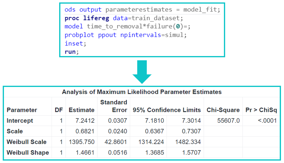
Figure 3 presents a code snippet demonstrating how to perform Weibull regression modeling with PROC LIFEREG for the data set illustrated in Figure 2. The input data come from the training data set train_dataset. The code line model time_to_removal*failure(0); assumes that failure = 0 represents the rows of the data set that are not associated with the failure events. The output is saved in the SAS data table model_fit, and it is presented in the lower half of Figure 3. We see that the Weibull distribution parameters, Weibull Shape and Weibull Scale, are estimated as 1.4661 and 1395.750, respectively, with standard errors of 0.0516 and 42.8601. Therefore, we are 95% confident that the Weibull shape parameter falls between 1.3685 and 1.5707, indicating wear-out failures (that is, degrading of the asset over time due to wear). Similarly, we are 95% confident that the Weibull scale parameter falls between 1314.224 and 1482.334. Furthermore, Weibull Scale = exp (Intercept) and Weibull Shape = 1/Scale.

Note that the best fit overlaying the histogram of the times to removal in Figure 2 is also a Weibull distribution but with shape and scale parameters that are 1.46 and 1003.52. The difference between the values of Weibull parameters estimated for the time to removal (Figure 2) and the time to failure (Figure 3) demonstrate the importance of accounting for censoring, that often exists in asset failure event data sets as we predict asset lifetimes.

Model assessment

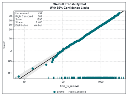
A way of assessing the goodness of the Weibull distribution fit identified in Figure 3 is via the use of the Weibull probability plot created by the command line probplot ppout npintervals=simul. The example plot obtained by using the training data set is presented in Figure 4. It shows that most of the data points fall within the 95% confidence bands. Thus, it is reasonable to model the training event data set by using the Weibull distribution function. A similar visualization can be created by using the test data set together with the same Weibull distribution fit.

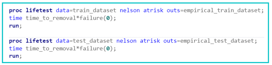
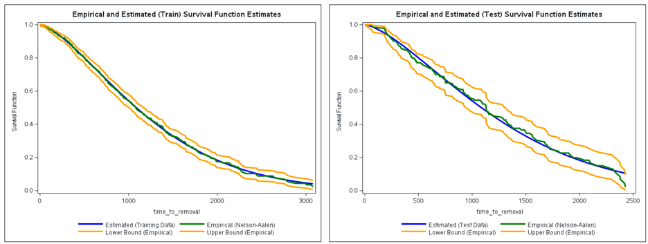
Figure 5: Creating the empirical (Nelson-Aalen) survival functions

An alternative way of assessing the goodness of the Weibull distribution fit is to compare the empirical (Nelson-Aalen) survival function with the estimated survival function for each of the training and test data sets. The empirical survival functions and their 95% confidence limits can be readily obtained by using PROC LIFETEST, as shown in Figure 5. The resulting empirical distribution functions are combined with the mean survival functions implied by the Weibull Scale and Weibull Shape parameter estimates in Figure 3. The corresponding mean survival functions can be obtained by evaluating the following SAS code line: EXP(-((time_to_removal/Weibull_Scale)**Weibull_Shape)).

Figure 6 presents the resulting comparison plots. We see that the estimated mean survival function (in blue) and empirical survival function (in green) mostly align with each other. Although the 95% confidence interval identified for the empirical survival function is wider for the test data set, all predictions fall between the confidence limits. Thus, both assessments agree on the suitability of the fitted Weibull distribution to approximate the lifetime distribution embedded into the historical right-censored event data set.

Figure 6: Comparison of empirical (Nelson-Aalen) distribution to the estimated survival function

Summary

This post starts with creating an event data set that can be readily used for asset lifetime prediction. We provide a step-by-step description of fitting a Weibull distribution function to the corresponding right-censored data with PROC LIFEREG and assessing the resulting model fit by comparing empirical and estimated survival probability functions with the help of PROC LIFETEST. Throughout, we focus on one asset only. However, our presentation here can be readily extended to any number of assets to characterize their individual lifetime distribution functions. Furthermore, the event data sets in Figure 2 and reliability modeling in Figure 3 can be extended to include operational asset attributes to enhance the accuracy of lifetime predictions.

Another natural next step is to utilize this post's asset lifetime predictions to optimize the management of spare-part inventory. Challenges of developing a spare-part inventory management solution include the need to optimize under uncertainty and the importance of optimizing the inventory at the fleet level.
We will address these advanced topics of reliability modeling in upcoming posts of our asset performance management series. Stay tuned!