In my first article on hyperparameter autotuning, I used a cake analogy to show how to use hyperparameter autotuning with Optuna and the sasviya.ml package in Python to improve detecting Higgs bosons in a particle accelerator. SAS Viya Workbench now supports hyperparameter autotuning in SAS code with a variety of different machine learning models, helping you achieve greater accuracy with less code. Remember how using Optuna was like asking Gordon Ramsay to critique our cake? In Python, we had to get him into the kitchen and tell him what to critique and how to critique it. This time, he’s already here and ready to yell at you.
Let’s take a look at the absolute minimum amount of code needed to perform hyperparameter autotuning with a gradient boosting model using SAS code.
proc gradboost data=sashelp.iris; autotune; target species / level=nominal; input _NUMERIC_; run; |
Yep. That’s it. It’s literally one extra line: autotune.
When you add this single line, SAS will run it through a genetic algorithm, partition it into a 70/30 train/validation split, run multiple parallel evaluations in a single iteration, and automatically stop after either 50 evaluations, 5 iterations, 10 hours, or stagnation in 4 iterations. Each hyperparameter has pre-configured default bounds and is fully modifiable. If you’re curious as to what these defaults are, check out the documentation for the AUTOTUNE statement in PROC GRADBOOST.
That’s a whole lot of things happening from that one little statement. This gives you a good baseline, and considering how well-tuned the default values are, it may end up being all you need.
Predicting Higgs bosons with SAS
Let’s go back to solving the Higgs boson prediction problem, and this time we’ll do it with SAS code. One thing I love about programming in SAS is how compact the code is for modeling. To show you how little code is needed to solve this problem in its entirety, I’m going to post the whole program below.
filename inpipe pipe "unzip -p /workspaces/myfolder/data/higgs.zip | gunzip -c"; %let colnames = signal lepton_pt lepton_eta lepton_phi missing_energy_magnitude missing_energy_phi jet_1_pt jet_1_eta jet_1_phi jet_1_btag jet_2_pt jet_2_eta jet_2_phi jet_2_btag jet_3_pt jet_3_eta jet_3_phi jet_3_btag jet_4_pt jet_4_eta jet_4_phi jet_4_btag m_jj m_jjj m_lv m_jlv m_bb m_wbb m_wwbb ; data higgs; infile inpipe dlm=',' dsd; input &colnames; drop m_:; run; proc gradboost data=higgs outmodel=low_level_model seed=42 earlystop(stagnation=0); partition fraction(validate=0.15 test=0.15 seed=42); autotune objective=auc searchmethod=bayesian targetevent='1' popsize=5 historytable=higgs_low_level_history tuningparameters = ( ntrees(UB=300) maxdepth(UB=30) learningrate(UB=0.1) ) ; target signal / level=nominal; input _NUMERIC_; output out=low_level_preds role; run; |
That’s a grand total of 38 lines, including some extra whitespace for readability. In those 38 lines, we:
- Define where our file is and how to unpack with unzip and gunzip:
filename inpipe pipe "unzip -p /workspaces/myfolder/data/higgs.zip | gunzip -c";
- Define our column names and their order:
%let colnames = ...;
- Unzip, untar, and read in the data:
data higgs;
    infile inpipe dlm=',' dsd;
    input &colnames;
    drop m_:;
run;
Then, in one gradient boosting procedure:
- Perform a repeatable train/validate/test split:
partition fraction(validate=0.15 test=0.15 seed=42)
- Enable autotuning:
autotune
- Set our autotuning objective, search method, and target event:
objective=auc searchmethod=bayesian targetevent='1' - Create 4 parallel evaluations, with 5 iterations and 5 evaluations per iteration:
popsize=5 - Save the best model, autotuning history, predictions, and tag the role of each prediction:
outmodel=low_level_model historytable=higgs_low_level_history output out=low_level_preds role - Set a few hyperparameter bounds to try because we learned last time that more trees, lower depth, and a lower learning rate are important with this data:
tuningparameters = (
    ntrees(UB=300)
    maxdepth(UB=30)
    learningrate(UB=0.1)
)
Even though we changed the bounds of a few of our hyperparameters, we are still tuning the rest of the parameters as well. We just gave it some more suggestions.
There are a ton of other autotuning options available. We can go much further than this, including excluding hyperparameters from tuning, adding a second objective, setting a maximum time, using k-fold cross validation, setting a stagnation threshold, and much more.
Not only that, but PROC GRADBOOST handles both classification and regression in only one PROC. You simply tell it what type of target you have, and it sorts out the rest. You’ll find this to be the case for the rest of the machine learning PROCs too, such as Deep Neural Networks and Support Vector Machines. This simplifies the world of models you need to know.
Let’s run this model and see how it compares.
The results
How did we do this time around? Using the SAS autotuning framework, we achieved a test AUC of 0.801 for the low-level model. Let’s put this into perspective with the rest of the models we were against, including our previous SAS model that was tuned with Optuna.
| Model | AUC: Low-level | Δ vs SAS (%) |
| SAS: Tuned Gradient Boosting | 0.801 | |
| SAS: Tuned Gradient Boosting (Optuna) | 0.795 | -0.75% |
| Paper: Boosted Decision Tree | 0.73 | -8.9% |
| Paper: Shallow Neural Network | 0.733 | -8.5% |
| Paper: Deep Neural Network | 0.880 | +9.9% |
Here’s what all the evaluations looked like:
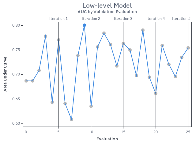
Overall, impressive results for how little code we needed, and we even got our best result just 9 evaluations in. This shows how well SAS has tuned its hyperparameter autotuning framework, looking at optimal combinations of hyperparameters to test without the end-user trying to find a good starting point for each one.
Going bigger
If you’re ready to scale out with huge data, you don’t need to learn a whole new language. Many SAS modeling procedures automatically change where the calculations happen, bringing massively parallel, multithreaded processing to your data without any extra effort on your part. All you need to do is load your data to CAS and change your input dataset, then SAS handles the rest.
Don’t believe me? Give it a try yourself on SAS Viya with our first example using Iris:
cas; caslib _ALL_ assign; data casuser.iris; set sashelp.iris; run; proc gradboost data=casuser.iris; autotune; target species / level=nominal; input _NUMERIC_; run; |
All we did was load the data into CAS and tell PROC GRADBOOST that our data is no longer on disk, but in CAS. Just like that, the processing is now massively parallel and ready to scale to your demands.
Wrapping it up
We went through two examples of using sasviya.ml’s GradientBoostingClassifier and PROC GRADBOOST, showing that you can get impressive results in either language. You may be wondering which one is better.
Want to know a secret?
They’re both using the exact same engine.
sasviya.ml isn’t some watered down set of algorithms for Python data scientists. Far from it. This is the same high-performance, trusted, battle-tested math that backs other SAS Viya machine learning models. The SAS Viya Python API is designed to be Pythonic and work with other open source packages, letting you seamlessly integrate your favorite packages in the open source ecosystem, like Optuna, with virtually no learning curve.
The flexibility of SAS Viya Workbench gives you the option to run your models in multiple languages while using the same underlying engine. Whether you’re using Python or a PROC, you can be assured that you’re going to get the performance and results that you expect from SAS. The language you use, and how you mix them together, is entirely up to you.
Links
- Previous article: Boost ML accuracy with hyperparameter tuning (with a fun twist)
- Documentation: Overview of Hyperparameter Autotuning in SAS Viya
- UC Irvine Machine Learning Repository - Higgs boson dataset
References
- Whiteson, D. (2014). HIGGS [Dataset]. UCI Machine Learning Repository. https://doi.org/10.24432/C5V312. Licensed under CC BY-SA 4.0.