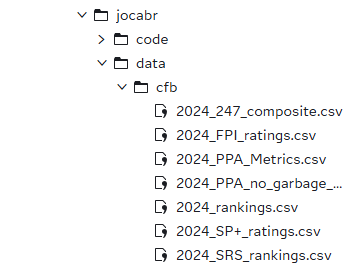
There's a chill in the air through much of the United States, and that can only mean one thing: the cold disappointment of your college football season as your team's playoff hopes fade away into the darkness. Back in September, I was curious about what data was readily available surrounding the CFB landscape: recruiting, rankings, gametime statistics, etc. Thanks to the brilliant data collection and export tools produced by CollegeFootballData.com, I was able to build a personalized series of datasets describing several areas of interest:

I was originally eyeing a predictive pipeline where I would use SAS Viya to make predictions on the season, but as the games distracted me from my code, I watched a wickedly entertaining (and arguably unlikely) season shake out before my eyes. I decided to pivot from a predictive approach to a more exploratory pipeline, and there's no better way to attack this than with SAS Viya's new ACCESS Engine to DuckDB. In this blog, I'll use my exploratory data analysis of college football data from the 2024-2025 off-season to highlight some neat features of DuckDB that can now be leveraged by the SAS/ACCESS Engine. Without further delay, let's dive into our data.
Data Ingestion
Before I start even viewing my datasets, I took the path of least resistance for ingestion and simply uploaded the datasets from my PC to the SAS Server on the Viya environment.
One neat capability of DuckDB is its versatility in connecting to data sources; if I were dealing with much larger scale datasets, I might have stored them on an S3 bucket, which SAS/ACCESS to DuckDB can query from with ease using DuckDB's installable extensions. That won't be the case here given the small-scale data at hand. As with any SAS pipeline, the first code we'll execute will set up a Library connection using the DuckDB Engine:
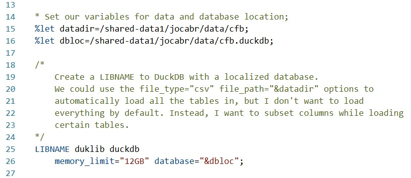
Like most SAS/ACCESS Engines, DuckDB LIBNAME statements have plenty of options for configuring your connection. In this case, all I've done is set an upper bound for the memory usage of the database and select a local path on the SAS Server for the DuckDB database file. A full list of options can be found here. Common configurations include the file_path and file_type options, which would instruct the library to load all files of a given type in the defined directory. I've opted against this as a best practice, since I don't want to load all my tables, nor will I want all the columns for every table. I'd rather only load what I need, when I need it—and DuckDB affords me that capability as well.
Loading And Exploring Our Tables
Based on what I exported from the College Football Database, I want to start with a "base table" of teams and their characteristics. Let's investigate the teams.csv table and see what we might want from it.
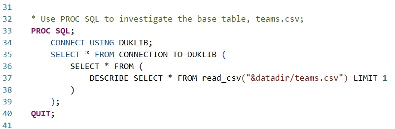
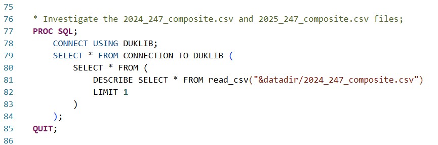
Using PROC SQL, I push-down a DESCRIBE SELECT * statement into the DuckDB instance, instructing it to tell me about the CSV dataset columns by just reading one line. In that sense, it's a SQL-writer's parallel to PROC CONTENTS.
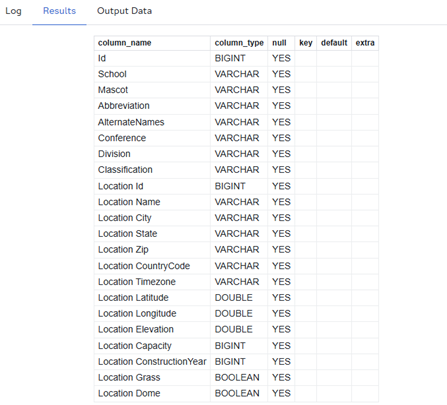
Well, that's a lot of columns, and I'm not sure I care about them all right now. Let's use PROC SQL to load what we want into the DUKLIB library:
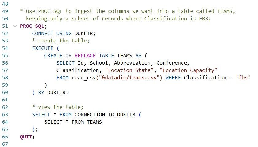
I'm doing a few different things in one procedure here. First, I use the CONNECT statement (as done previously) to tell SAS which data source to connect to (the DuckDB library, of course). The EXECUTE statement explicitly pushes SQL code down to DuckDB, meaning that I can write anything I want in DuckDB's flavor of SQL (closely related to the PostgreSQL dialect). This dialect allows us to leverage tons of features unavailable to the standard PROC SQL syntax. An easy but significant example here is the CREATE OR REPLACE syntax, which, if ran implicitly in PROC SQL on a standard SAS library, would not be recognized! This is obviously nice since I continually, without fail, forget to drop tables when I edit and re-run queries.
At the bottom of the query, the SELECT * FROM CONNECTION is used to generate an output in the SAS GUI. All EXECUTE statements do just as implied—they execute code in DuckDB—but their results aren't propagated back up to the SAS user interface. If you put a SELECT statement inside an EXECUTE statement, DuckDB would run it, but you, the SAS user, wouldn't see the results. Thus, the SELECT * FROM CONNECTION is what we use to retrieve results from a query.
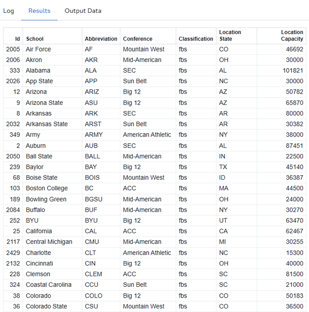
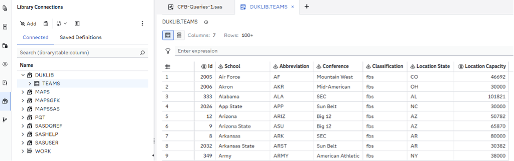
We now have a TEAMS table under DUKLIB, which we can see in our Library pane, just as we would with any other type of data source:
I've talked a lot for just loading a single table, but it's important to lay the groundwork of how the syntax works when using PROC SQL with DuckDB. The benefits are substantial, especially for large and easily subsettable datasets, but—as with any new tool—there’s a learning curve to mastering the syntax. Let's move on and focus on some more data.
Investigation #1: Talent Gain & Loss Over the Offseason
In the modern age of transfer portals, NIL, and ever-increasingly wild coaching carousels, the number one burning question I had of my data was "who gained and who lost talent over the offseason?" I'm not interested in just the transfers, but also the graduates and the incoming freshmen. I have two CSV files pertaining to this, 2024_247_composite.csv and 2025_247_composite.csv, containing data procured from the 247 sports news site.
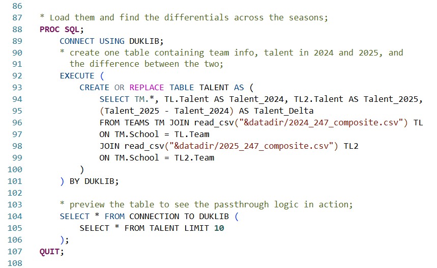
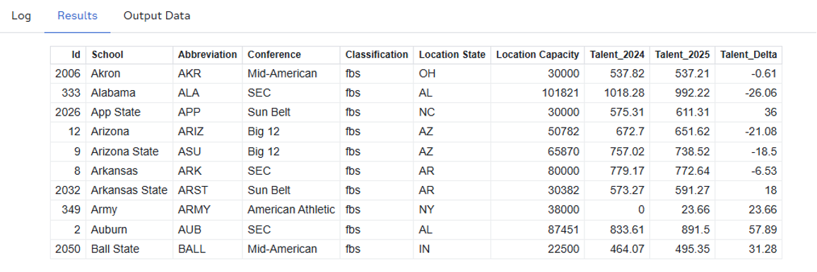
The first PROC SQL mimics what we did for the TEAMS dataset, and tells us we have three columns: “Year”, “Team”, and “Talent.” Knowing that we have two files, one for 2024 and one for 2025, I join BOTH tables to the DUKLIB.TEAMS table on account of team name, then create a calculated column, “Talent_Delta”, of the difference between the 247-assessed talent metrics. Lastly, I use a SELECT * FROM CONNECTION statement to preview my new dataset, DUKLIB.TALENT.
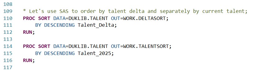
So far, everything I've done has been in PROC SQL, which makes sense, since DuckDB, after all, is operated with SQL. But can I leverage other PROC's from SAS' toolbox as I would with a different library connection? The answer is a resounding YES. Let's create two tables in our ephemeral WORK library by using PROC SORT on our DUKLIB.TALENT table, ordering our FBS teams by “Talent_Delta” in one output, and by “Talent_2025” in another.
Resulting DELTASORT Table:
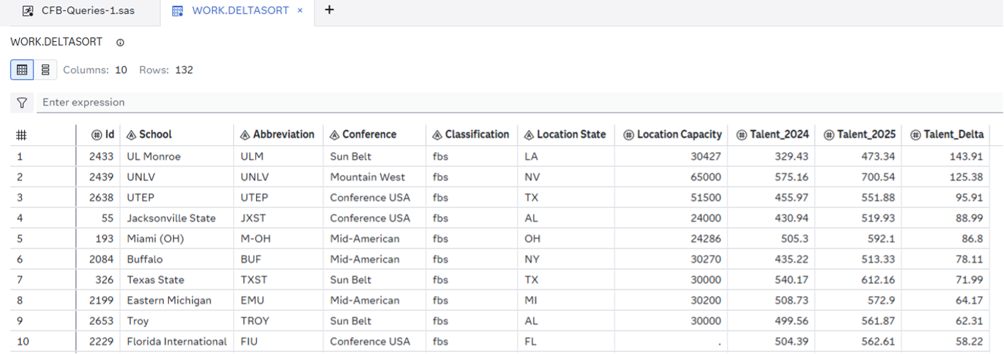
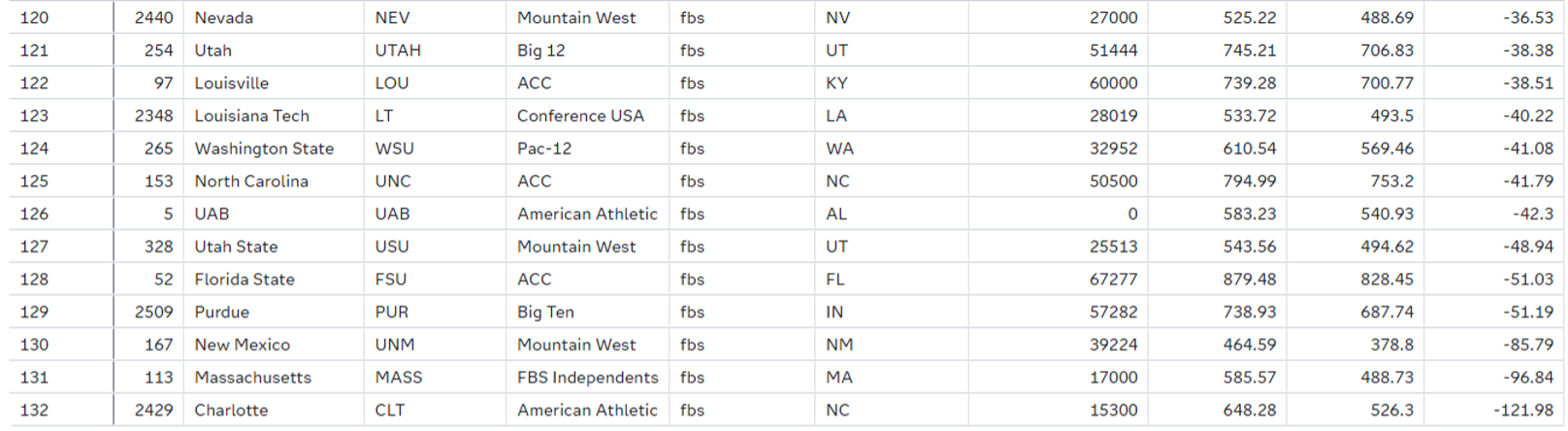
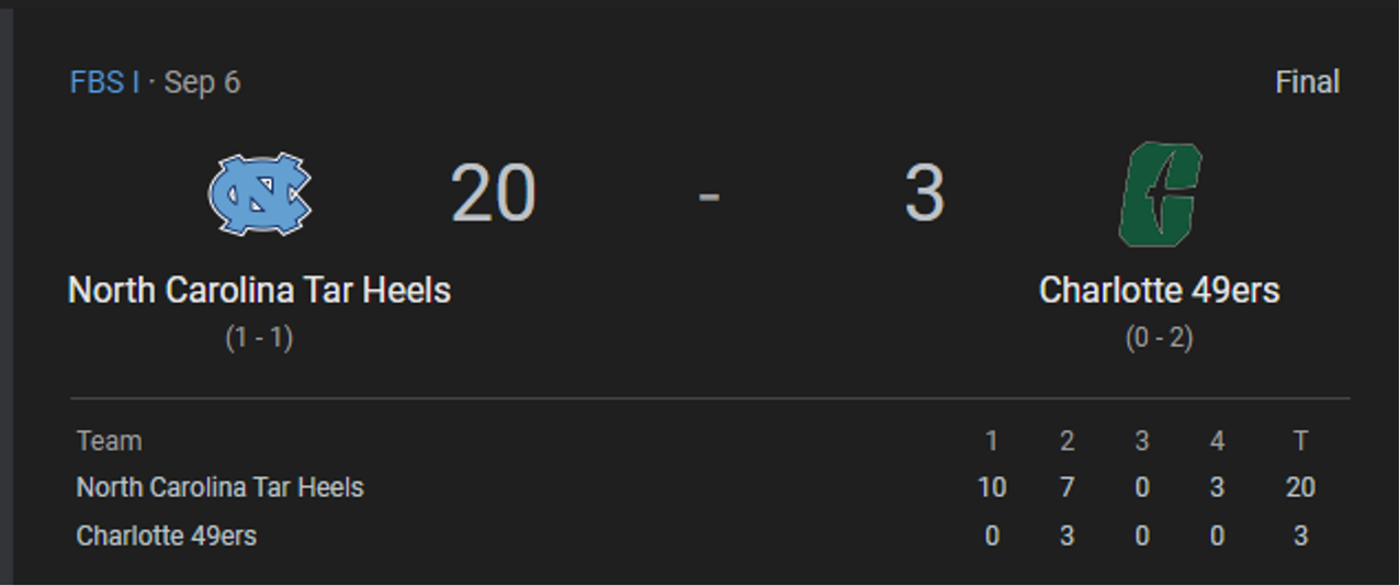
You would expect the big Power 4 names to top the DELTASORT table, but, as we'll see in the TALENTSORT table, it's hard to post such large gains when your team was already so talented AND losing players to graduation and transfers. Sympathies do go out to Charlotte, who rounds out the bottom after being virtually gutted over the offseason. Perhaps that partially explains their 1-9 record on the year:
In terms of raw talent, the familiar leaders emerge atop the TALENTSORT table:

Writing this blog across October and November, I find this simple sort shows the pure beauty of college football: talent doesn't guarantee anything. Check #6 LSU, or #9 Penn State, or #12 Auburn, or #13 Florida, all three of which have missed their expectations so significantly that they've paid millions of dollars just to get rid of their coaches. My condolences go to the fanbases, but after all, it's the suffering that builds character.
Investigation #2: Offseason Recruiting
With a general idea of who gained "talent" between seasons, let's dive deeper and focus on the actual recruiting process. Down the line, it would surely be interesting to line that data up next to a list of publicly known NIL funds. I'd bet on a strong correlation. Money talks, in the end.
Anyways, let's investigate the recruiting using the 2025_recruiting_detailed.csv dataset. Just as in the previous investigation, I'll use the DUKLIB connection to select the results of a DESCRIBE statement to get the metadata on our columns.
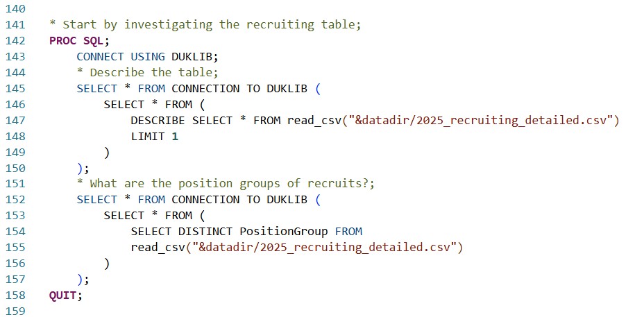
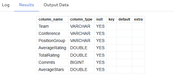
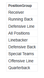
The number one thing that sticks out to me after running the DESCRIBE statement alone is the PositionGroup variable—what ARE the Position Groups of recruiting, anyway? The SELECT DISTINCT statement/clause will parse exactly that.
The results tell us we have eight total Position Groups, and a summative group as well. That means every team has multiple records pertaining to their recruiting efforts (number of commits, average rating of commits) in different Position Groups, along with a cumulative record. I could simply use a WHERE clause to pull the cumulative records only, but that's no fun, and we'd lose plenty of valuable information—even though we don't need data to see that your school forgot to recruit a quarterback. Thankfully, DuckDB provides a key functionality that will allow us to transform this tall dataset into a wide format that will join one-to-one cleanly with our teams & talent data. Let's start by binning some of the Position Groups into categories:
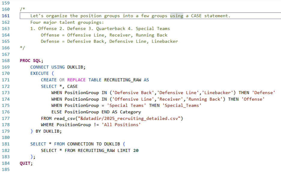
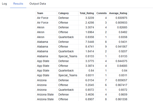
The CASE clause within the EXECUTE statement does exactly what SQL programmers (and Python programmers alike) would expect—it buckets different situations into different results, and saves those results to a new column, called "Category." Here, we isolate four main categories, which closely align with the "three phases of the game": under Defense, we keep "Defensive Back," "Defensive Line," and "Linebacker." Under Offense, we keep "Offensive Line," "Receiver," and "Running Back." Quarterback and Special Teams get their own categories, the former of which could easily slot under Offense, but might be worth considering as its own entity due to its sheer impact on a team's performance. Here's what our DUKLIB.RECRUITING_RAW table looks like:
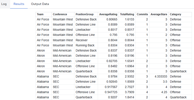
We haven't consolidated any records yet, but we can see the Category attributed to each record, and we can see that not every team has data in every position. Air Force, as seen above, has no data on Quarterback recruiting. There's some irony and a piloting joke in there, I'm sure of it.
In our next step, we introduce DuckDB functions, which match many of the push-down functions that PROC SQL can leverage in-database with different data sources. We are using explicit passthrough here to leverage DuckDB's functions themselves but note that an implicit passthrough query could leverage many of these same functions.
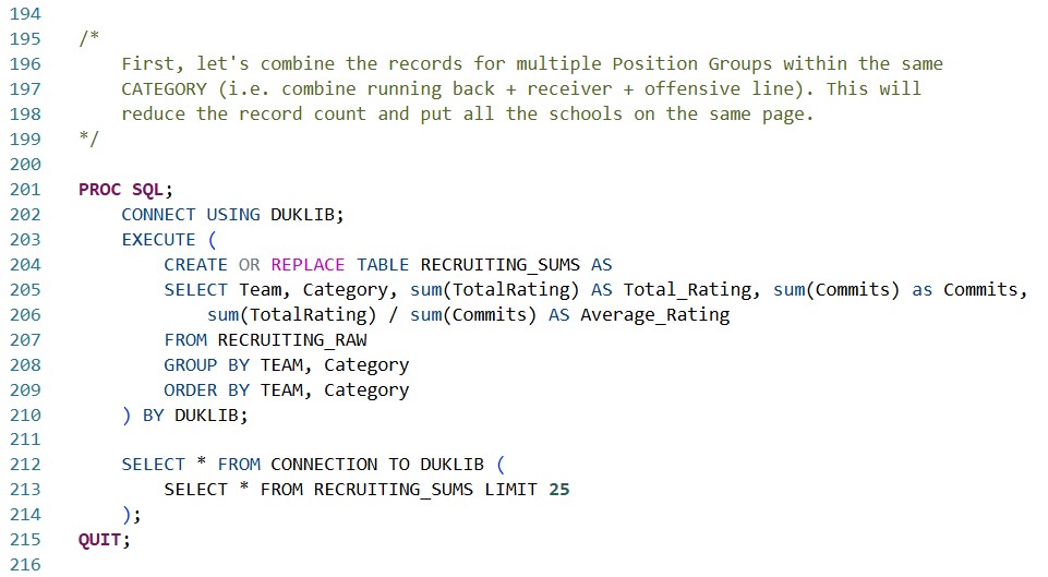
We've now consolidated our data into a maximum of four records per team: Defense, Offense, Quarterback, and Special_Teams using the sum() functions in DuckDB, and leveraging our GROUP BY and ORDER BY statements to keep everything lined up nicely.
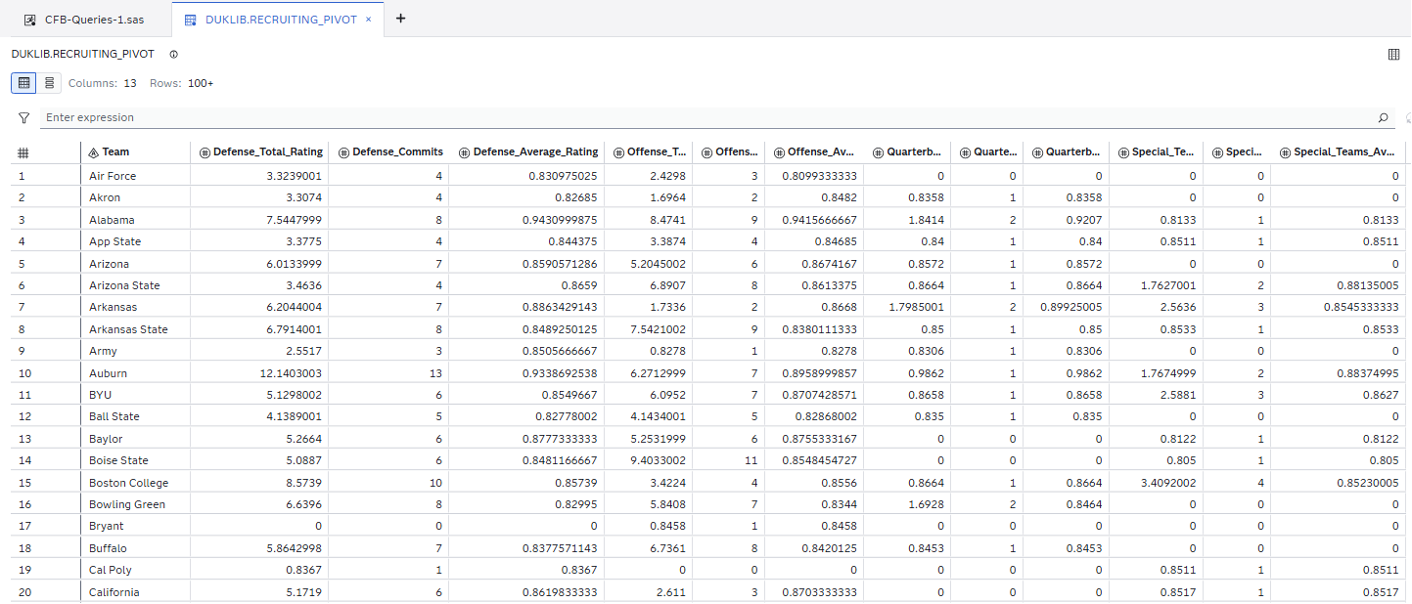
With this consolidation done, we can introduce the highlight DuckDB feature of this article, something that can't be done using ANSI Standard PROC SQL: the PIVOT statement. The PIVOT statement in DuckDB, in conjunction with DuckDB's coalesce() function, allows us to restructure our data in one SQL statement, combining multiple records into multiple columns, grouped by the team.
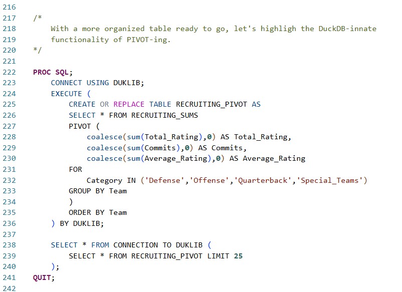
Our newest table, DUKLIB.RECRUITING_PIVOT, now contains just a single record per team, with clearly named columns defining the number of commits, total rating, and (more importantly) average rating in each major category of the game.
The PIVOT statement is a powerful piece of logic that is now accessible to all SAS Viya programmers working with the SAS/ACCESS Engine to DuckDB. It's only one of many benefits that the newly introduced ACCESS Engine brings to the programmer experience, but it highlights SAS' paradigm of meeting your data where it is.
In my next article, I'll highlight more neat features that PROC SQL can take advantage of with DuckDB, and I'll engage a few more of our football datasets, updated for the end of the regular season, remarking along the way on how drastically the 2025 season's results have deviated from the expectations. In the meantime, you can learn more about SAS/ACCESS to DuckDB in SAS Viya 4 here.
Thanks for reading, and I'll see you in ten yards.

2 Comments
Great write up Joe! Go Miami!
Love this Joe! Great work and write up!