When generating animation files, the number of frames shown per second is called the frame rate (FPS - Frames per second). Generally, the higher the frame rate, the smoother the animation. Human eyes can process 10 to 12 frames per second and perceive them individually, while higher frame rates are perceived as motion due to "persistence of vision." Modern movies are usually shot and presented at 24 FPS, and there are currently five commonly used frame rates in the film and television industry: 24 FPS, 25 FPS, 30 FPS, 50 FPS and 60 FPS for HDTV.

Animations can present richer time-varying analysis results than static images. It can consider and compare analysis results from different angles to present more details. Animations generated in SAS can be in GIF or SVG format. Various SAS/Graph PROC and SG PROC steps support generating animated GIF files. This short post discusses some timing control issues that authors have found while generating animations for rigorous physics simulations with SAS. Preserving time accuracy is important in physics simulation and some time-sensitive animation generation.

GIF format review

The Graphics Interchange Format (GIF) is a bitmap image format with animation features created by CompuServer in 1987, and GIF89a is version 89a (July 1989) of the format. Its advantages include smaller file sizes and wider support for web browsers and platforms, but the smallest unit of frame duration in the GIF89a file format is hundredths of a second (0.01 seconds) instead of milliseconds (0.001 seconds). Many GIF tools allow specifying the frame duration in milliseconds, even though they will be rounded to hundredths of seconds anyways. They unintendedly mask the limitations of this file format. On the other hand, some GIF-playing software will automatically modify a time interval that is too small. For example, Microsoft's IE rounds up time intervals under 50ms to 100ms. This creates certain challenges for producing time-accurate animations.

Research in 2014^[1] indicated that GIF89a does not produce substantial delays when an animation interval is larger than 100ms, regardless of the web browser. Below this threshold, the resulting performance falls considerably. IE9 reinterprets any delay below 100ms as 100ms, so a 50ms interval shows a 50ms delay, while a 16.67ms interval shows around 85ms delay. Firefox 10 and Chrome 17 can execute a GIF89a animation correctly (except for an 85ms delay on 16.67ms intervals), and their mean number of missed frames is smaller and stabilizes over time. The refresh interval is 16.67 milliseconds for a screen with a refresh rate of 60Hz.

Due to the need to control the size of the generated file, 8 FPS (125ms) is enough for most GIF files. When there are many dynamics at play, we can use 15 FPS (66.67ms). The file size for 24 FPS (41.67ms) GIFs without compression will be larger than a standard MP4 video file, so then it would be better to produce the animation as an MP4 instead of a GIF format with a higher FPS.

What is the proper FPS?

When generating animations in SAS, you can specify the duration of a frame through the SAS system option ANIMDURATION. It can accept up to 10 characters in length, that is, there can be 8 significant digits after the decimal point. This commonly leads to programmers incorrectly thinking that the duration of the animation can be specified in milliseconds. The actual test shows that in SAS, the duration of a frame specified via ANIMDURATION option with value 1/FPS, and the actual duration of the animation will be quite different. That is, if the programmer wants to generate relatively time-accurate animation directly in the simulation, they should pay attention when selecting a specific FPS to generate the animation and use the following relationship to specify the target DURATION value:

/*Calculate the accurate ANIMDURATION from/to FPS in SAS*/
 
proc fcmp inlib=work.proto outlib=work.fcmp.animation;
  function fps_animduration(fps);
    dur=1/fps;
    return( floor( dur * 100)/100 ); *Keep the first 2 digits after decimal point instead of round(dur, 0.01);
  endsub;
 
  function animduration_fps(dur);
    return( floor(<strong>1</strong>/dur) ); *Cut the integer part;
  endsub;
run;
 
option cmplib=(work.fcmp);

Accordingly, the following conversion can be used in SAS Macro:

%let DUR=%sysevalf( %sysfunc(floor((1/&FPS)*100 ))/100 );

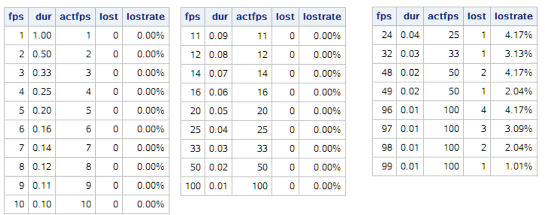
In a time-accurate physics simulation, the duration or period is the absolute time, so the number of frames that need to be generated is the duration divided by the frame rate. Since the minimum unit of GIF per frame duration mentioned above is one-hundredth of a second, the actual generated frame rate is larger than expected in a generated GIF file, which means that the actual number of frames generated is less than expected for a specified simulation duration. Experiments show that when the FPS is less than or equal to 100, if no error in the number of generated frames is allowed, there are only 19 frame rates that can be used: 1-10, 11, 12, 14, 16, 20, 25, 33, 50 and 100 FPS. If 5% of the generated frames or time error is allowed, you can have an additional 8 frame rates to choose from: 24, 32, 48, 49, 96, 97, 98 and 99 FPS. Based on the background knowledge mentioned earlier, combined with actual needs, GIF file size limitations and playback smoothness requirements, we’d better generally choose a frame rate between 8 and 25 to produce time-accurate animations. 8, 10, 16, 20 and 25 FPS are all good choices. 24 FPS can be chosen if the error rate of frames generated is allowed to be <=5%. The following table lists the error between the actual number of frames generated and the expected number of frames when the duration is 1s under different FPS settings:

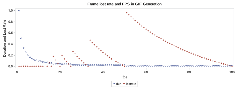
The relationship between the actual loss rate of generated frames and specified FPS in the figure below reveals which frame rate we should specify when generating time-accurate animations:

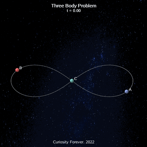
The figure below is a single-cycle animation generated by solving the figure-8 solution of the three-body problem in SAS. The physical time of a single cycle is about 6.3259 seconds, and the actual animation time is also 6.32 seconds with a time scale factor of 1. The duration is 0.04s per frame, for a total of 158 frames. In fact, the problem discussed in this article was discovered when trying to solve the three-body problem with SAS. Of course, in addition to the above frame rate selection, introducing compression techniques to SAS GIF generating is recommended to reduce the file size. Several experiments have shown that third-party tools such as GIF Optimizer can be used to reduce a GIF file's size by 90% without a significant reduction in graphics quality.

Conclusion

When generating GIF animations in SAS that need to be time-accurate such as physics simulation, pay attention to the selection of the ANIMDURATION corresponding to the appropriate frame rate. When programming a GIF animation to display the analysis results, do not choose a random frame rate, or else there will be a large loss of generated frames or a time error. 8, 10, 16, 20 and 25 FPS can be chosen when there is no generated frame loss allowed and 24 FPS can be selected when a generated frame loss rate below 5% is allowed. The limitations discussed here are inherent to the GIF file specification; not due to SAS or third-party tools.

Learn more

• Creating Animated GIF Images and SVG Documents
• Animating Images in SAS/GRAPH
• Examples: Generating Animated Images