Partition your CAS tables to greatly improve performance

When you execute code on the SAS® Cloud Analytic Services (CAS) server, one way you can improve performance is by partitioning a table. A partitioned table enables the data to load faster when that data needs to be grouped by the common values of a variable.

This post explains what it means to partition a table and describes the advantages of a partitioned table. I'll illustrate these concepts with example code that shows improved processing time when you use a partitioned table.

SAS BY-group requires SORT

BY-group processing enables you to group your data by unique variable values. This processing is used, for example, in tasks like merging data sets by a common variable and producing reports that contain data that is grouped by the value of a classification variable. You also use BY-group processing when you execute code in CAS. A key difference in creating BY-groups in SAS versus in CAS is that SAS requires a SORT procedure to sort the data by the specified BY variable in order to create the BY groups.

BY-group sorting implicit in CAS

This step is not required in CAS. When you perform BY-group processing on a CAS table, an implicit sorting action takes place, and each BY-group is distributed to the available threads. This implicit sort process takes place each time that the table is accessed and the BY-groups are requested.

Partitioning a CAS table permanently stores the table such that the values of the BY variable are grouped. Using a partitioned CAS table enables you to skip the implicit sort process each time the table is used, which can greatly improve performance.

Partition CAS action example

You create a partitioned CAS table by using the partition CAS action. The following example shows how to partition the CARS table (created from the SASHELP.CARS data set) by the MAKE variable.

caslib _all_ assign;    ①
data casuser.cars;      
set sashelp.cars;  ②
run;
proc cas;
table.partition /     ③                                              
casout={caslib="casuser", name="cars2"} ④                            
table={caslib="casuser", name="cars", groupby={name="make"}}; ⑤
quit;

In this code:

① The CASLIB statement creates SAS librefs that point to all existing caslibs. CASUSER, which is used in the subsequent DATA step, is one of the librefs that are created by this statement.

② The DATA step creates the CARS CAS table in the CASUSER caslib.

③ The partition action in the CAS procedure is part of the TABLE action set.

④ The casout= parameter contains the caslib= parameter, which points to the caslib where the partitioned CAS table named CARS2 will be stored.

⑤ The table= parameter contains the name= parameter, which lists the name of the table that is being partitioned. It also contains the CASLIB= option, which points to the caslib in which the table is stored. The groupby= parameter contains the name= option, which names the variable by which to partition the table.

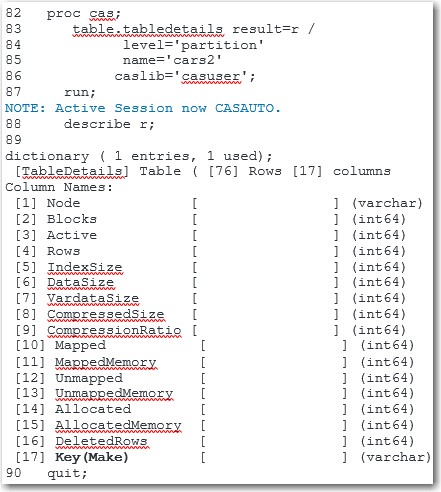
You can confirm that the table has been partitioned by submitting the following CAS procedure with the tabledetails action.

proc cas;
table.tabledetails result=r / level='partition' ①
name='cars2'
caslib='casuser';
run;
describe r; ②
quit;

In this code:
① The LEVEL= parameter specifies the aggregation level of the TABLEDETAILS output.
② The DESCRIBE statement writes the output of the TABLEDETAILS action to the log.

The following output is displayed in the resulting log. The KEY column shows the variable the table has been partitioned by.

As mentioned earlier, the purpose of partitioning a table is to improve performance. The following example uses two CAS tables that consist of an ID variable with 10 possible values and 10 character variables. Each table contains 5,000,000 rows. This example illustrates how much performance improvement you can gain by partitioning the tables. In this case, the ID variable merges two tables.

First, you create the tables by submitting the following DATA steps:

data casuser.one;
array vars(10) $8 x1-x10;
do j=1 to 5000000;
id=put(rand('integer',1,10),8.);
do i=1 to 10;
vars(i)=byte(rand('integer',65,90));
end;
output;
end;
drop i j;
run;
 
data casuser.two;
array vars(10) $8 x1-x10;
do j=1 to 5000000;
id=put(rand('integer',1,10),8.);
do i=1 to 10;
vars(i)=byte(rand('integer',65,90));
end;
output;
end;
drop i j;
run;

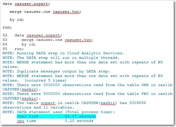
The DATA steps above show how to merge non-partitioned tables. In the log output shown below, you can see that the total, real time (highlighted) took almost 45 seconds to run.

Partitioned tables example

The next example runs the same DATA step code, but it uses partitioned tables. The first step is to partition the tables, as shown below:

proc cas;
table.partition /                                                   
casout={caslib="casuser", name="onepart"}                             
table={caslib="casuser", name="one", groupby={name="id"}};   
run; 
 
table.partition /                                                   
casout={caslib="casuser", name="twopart"}                             
table={caslib="casuser", name="two", groupby={name="id"}};   
quit;

To merge the two tables and to product the log, submit the following code. (The real time is highlighted in the log.)

data casuser.nopart;
merge casuser.onepart casuser.twopart;
by id;
run;

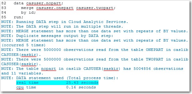
The output for this code is show below:

This time, the DATA Step took only 25.43 seconds to execute. That is a 43% improvement in execution time!

Partition for improved performance

If your analysis requires you to use the same table multiple times to perform BY-group processing, then I strongly recommend that you partition the table. As the last example shows, partitioning your table can greatly improve performance!

Blogs