With time series data analysis, we can apply moving average methods to predict data points without seasonality. This includes Simple Average (SA), Simple Moving Average (SMA), Weighted Moving Average (WMA), Exponential Moving Average (EMA), etc. For series with a trend but without seasonality, we can use linear, non-linear and autoregressive prediction models. In practice, we often use these kinds of moving average methods for series data with large variance, e.g. financial and stock market data.

Since introducing the window concept, SMA reflects historical data with a lag problem, and all points in the same window have the same importance to the current point. Weights are introduced to reflect the different importances of points in a window, and it leads to WMA and EMA. WMA gives greater weight to recent observations while less weight to the longer-term observations. The weights decrease in a linear fashion. If the sequence fluctuations are not large, the same weight is given to the observation and WMA degenerates into a SMA and the WMA becomes an EMA when weights decrease exponentially. However, these traditional moving average methods ave a lag problem due to introducing the smooth window concept and its results are less responsive to the current value. To gain a better balance between lag reduction and curve smoothing in a moving average, we must get help from some smarter mathematics algorithm.

What is Hull Moving Average?

Hull Moving Average (HMA) is a fast moving average method with low lag developed by Australia investor Alan Hull in 2005. It’s known to almost eliminate lag altogether and manages to improve smoothing at the same time. Longer period HMAs can be used as an indicator to identify trend, and shorter period HMAs can be used as entry signals in the direction of the prevailing trend. Due to lag problems in all moving average methods, it’s not suggested to be used as a reverse signal alone. Anyway, we can use different window HMAs to build a more robust trading strategy. E.g., 52-week HMA for trend indicator, and 13-week HMA for entry signal. Here is how it works:

• Long period HMA identifies the trend: rising HMA indicates the prevailing trend is rising, it’s better to enter long positions; falling HMA indicate the prevailing trend is falling, it’s better to enter short positions.
• Short period HMA identifies the entry signals in the direction of the prevailing trend: When the prevailing trend is rising, HMA goes up to indicate a long entry signal. When the prevailing trend is falling, HMA goes down to indicate a short entry signal.

Both long & short period HMAs in bullish mode generate Long Signal, and both in bearish mode generate Short Signal. So Long Trades get a buy signal after a Long Signal occurs, while Short Trades get a sell signal after a Short Signal occurs. Long Trades get a Sell Signal when Long or Short Trend is no longer bullish and Short Trades get a buy signal when Long or Short trend is no longer bearish. Figure 1 is a sample for this HMA based trading strategy.

In fact, HMA is quite simple. Its calculation only includes three WMA steps:

1. Calculate WMA of original sequence X using window length n ;
2. Calculate WMA of X using window length n/2;
3. Calculate WMA of derived sequence Y using window length Sqrt(n), while Y is the new series of 2 * WMA(x, n/2) – WMA(x, n). So HMA(x, n) formula can be defined as below:

HMA(x, n) = WMA( 2*WMA(x, n/2) − WMA(x, n), sqrt(n) )

HMA makes the moving average line more responsive to current value and keeps the smoothing of the curve line. It almost eliminates lag altogether and manages to improve smoothing at the same time.

How does HMA achieve the perfect balance?

We know SMA can gain the curve line of an average value for historical data falling in the current window, but it has the constant lag of at least a half window. The output may also have poor smoothness. If we embed SMA multiple times to get the average of the averages, it would be smoother but would increase lag at the same time.

Suppose we have this series: {1, 2, 3, 4, 5, 6, 7, 8, 9, 10}. The SMA at the last point is 5.5 with window length n=10, i.e. SUM[1...10]/10
is much different than the real value 10. If we reduce the window length to n=5, the SMA at the last point is 8, i.e. SUM[6…10]/5. If we have the second SMA with half size window and add the difference between these two SMAs, then we can get 8 + (8-5.5)=10.5, which is very close to the real value 10 and will eliminate lag. Then we can use SMA with specific window length again to reduce that slight overcompensation and improve smoothness. HMA uses linear WMA instead of SMA, and the last window length is sqrt(n). This is the key trick with using HMA.

Figure 2 below shows the difference between HMA(x, 4) and embed SMA twice SMA( SMA(x,4),4).

In stock trading, there are lots of complicated technical indicators derived from stock historical data, such as Ease of Movement indicators (EMV), momentum indicators (MTM), MACD indicators, Energy indicator CR, KDJ indicators, Bollinger (BOL) and so on. Its essence is like feature engineering extraction before neural network training. The fundamental purpose is to find some intrinsic property from price fluctuation. The Hull moving average itself was discovered and applied to real trading practices, which gives us a glimpse to the complication of building an automatic financial trading strategy under the veil. It’s just the beginning, the reflex in trading and aging of models may both bring uncertainty, so the effectiveness of quantitative trading strategies is a very complex topic which needs to be validated through real practice.

HMA in SAS Code

SAS was created for data analysis however, and my colleagues go into detail about how data analysis connects with HMA. Check out Cindy Wang's How to Calculate Hull Moving Average in SAS Visual Analytics and Rick Wicklin's The Hull moving average: Implement a custom time series smoother in SAS. I would like to share how to implement both HMA/WMA with only 27 lines of code in this article. You can use the macro anywhere to build HMA series with specific window lengths.

First, implement Weighted Moving Average (WMA) with SAS macro as shown below (only 11 lines). The macro has four arguments:

• WMA_N       WMA window length
• INPUT          Input variable name
• OUT             Output variable name, default is input name with _WMA_n suffix
• OUTLABEL The label of output variable, default is “input name WMA(n)”

%macro AddWMA(WMA_N=4, INPUT=close, OUT=&INPUT._WMA_&WMA_N., OUTLABEL=&INPUT. WMA(&WMA_N.));
  retain _sumx_&INPUT._WMA_&WMA_N.;
  _sumx_&INPUT._WMA_&WMA_N.=sum (_sumx_&INPUT._WMA_&WMA_N., &INPUT., -lag&WMA_N.( &INPUT. )) ;
 
  retain _sum_&INPUT._WMA_&WMA_N.;
  _sum_&INPUT._WMA_&WMA_N.=sum (_sum_&INPUT._WMA_&WMA_N., &WMA_N * &INPUT., -lag( _sumx_&INPUT._WMA_&WMA_N.  )) ;
 
  retain _sumw_&INPUT._WMA_&WMA_N.;
  if _N_ <= &WMA_N then _sumw_&INPUT._WMA_&WMA_N. = sum (_sumw_&INPUT._WMA_&WMA_N., &WMA_N, -_N_, 1);
 
  &OUT=_sum_&INPUT._WMA_&WMA_N. / _sumw_&INPUT._WMA_&WMA_N.;
 
  drop _sumx_&INPUT._WMA_&WMA_N. _sumw_&INPUT._WMA_&WMA_N. _sum_&INPUT._WMA_&WMA_N.;
  label &OUT="&OUTLABEL"; 
%mend;

We must watch out for the trick in the upper implementation of WMA with linear weights. In fact, there is no do-loop in the code, and it also doesn’t perform repeat computations for weights and values. We just keep the last sum of all values in the window (See Ln2-3), and the sum for WMA is the last sum for WMA plus window length times the value subtracted from it (See Ln4-5). For weight sum computation, we just need to pay attention to the points less than the window length(See Ln6-7).

Second, implement HMA with three times WMA invocation as below, (only 9 lines). The macro has four arguments:

• HMA_N       HMA window length
• INPUT         Input variable name
• OUT            Output variable name, default is input name with _HMA_n suffix
• OUTLABEL The label of output variable, default is “input name HMA(n)”

%macro AddHMA(HMA_N=5, INPUT=close, OUT=&INPUT._HMA_&HMA_N., outlabel=&INPUT. HMA(&HMA_N.));
  %AddWMA(WMA_N=&HMA_N, INPUT=&INPUT.);
 
  %AddWMA(WMA_N=%sysfunc(round(&HMA_N./2)), INPUT=&INPUT.);
 
  &INPUT._HMA_&HMA_N._DELTA=2 * &INPUT._WMA_%sysfunc(round(&HMA_N./2))  - &INPUT._WMA_&HMA_N;
  %AddWMA(WMA_N=%sysfunc(round(%sysfunc(sqrt(&HMA_N)))), INPUT=&INPUT._HMA_&HMA_N._DELTA);
 
  rename &INPUT._HMA_&HMA_N._DELTA_WMA_%sysfunc(round(%sysfunc(sqrt(&HMA_N.))))=&OUT;
  label &INPUT._HMA_&HMA_N._DELTA_WMA_%sysfunc(round(%sysfunc(sqrt(&HMA_N.))))="&outlabel"; 
 
  drop &INPUT._WMA_&HMA_N &INPUT._WMA_%sysfunc(round(&HMA_N./2)) &INPUT._HMA_&HMA_N._DELTA;
%mend;

The upper code is very intuitive as the first two lines perform WMA with window n and n/2 for X, then the next two lines generate new series Y and performs WMA with window sqrt(n). Other codes are just to improve macro flexibility and to drop temp variables, etc.

To compare HMA with SMA result, we must also implement SMA with the 7 lines of code as shown below. It has the same argument as WMA/HMA above, but SMA is an unnecessary part of HMA macro %ADDHMA implmentation.

%macro AddMA(MA_N=5, INPUT=close, out=&INPUT._MA_&MA_N., outlabel=&INPUT. MA(&MA_N.));
  retain _sum_&INPUT._MA_&MA_N.;
  _sum_&INPUT._MA_&MA_N.=sum (_sum_&INPUT._MA_&MA_N., &INPUT., -lag&MA_N.( &INPUT. )) ;
  &out=_sum_&INPUT._MA_&MA_N. / min(_n_, &MA_N.);
 
  drop _sum_&INPUT._MA_&MA_N.;
  label &out="&outlabel";
%mend;

Now we can test all the above implementations as shown below. First is a simple case we described above:

data a;
  input x @@;
  %AddMA( input=x, MA_N=5, out=SMA, outlabel=%str(SMA)); 
  %AddHMA( input=x, HMA_N=5, out=HMA, outlabel=%str(HMA))  
datalines;
1 2 3 4 5 6 7 8 9 10
;
proc print data=a label;
  format _all_ 8.2;
run;

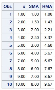
The output is listed below, the HMA result is much more close to the real value x than SMA. It’s more responsive and less in lag.

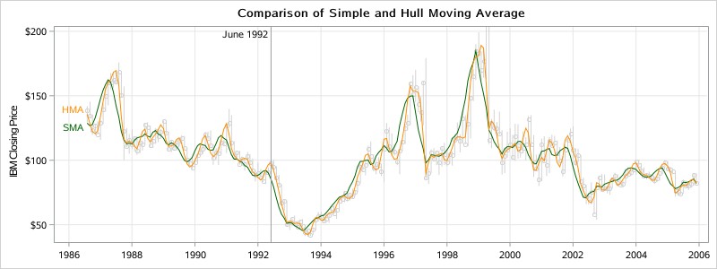
Now we can use the HMA macro to check IBM stock data in the SAS system dataset SASHELP.Stocks and draw trends in the plot to compare HMA(x, 5) and SMA(x, 5) output.

data Stocks_HMA;
  set sashelp.Stocks(where=(stock='IBM'));
  %AddHMA( HMA_N=5, out=HMA, outlabel=%str(HMA))
  %AddMA(MA_N=5, out=SMA, outlabel=%str(SMA));
run; 
ods graphics / width=800px height=300px;
title "Comparison of Simple and Hull Moving Average";
proc sgplot data=Stocks_HMA noautolegend;
   highlow x=Date high=High low=Low / lineattrs=(color=LightGray);
   scatter x=Date y=Close / markerattrs=(color=LightGray);
   series x=Date y=SMA / curvelabel curvelabelattrs=(color=DarkGreen) lineattrs=(color=DarkGreen);
   series x=Date y=HMA / curvelabel curvelabelattrs=(color=DarkOrange) lineattrs=(color=DarkOrange);
   refline '01JUN1992'd / axis=x label='June 1992' labelloc=inside;
   xaxis grid display=(nolabel); 
   yaxis grid max=200 label="IBM Closing Price";
run;

Summary

We have talked about what Hull Moving Average is, how it works, and worked through a super simple SAS Macro implementation for HMA, WMA and SMA with only 27 lines of SAS code. You can access the SAS code file directly through GitHub. This HMA implementation makes it quite simple and efficient to calculate HMA in SAS Data step without SAS/IML and Visual Analytics. In fact, it shows how easy process rolling-window computation for time series data can be in SAS, and opens a new window to build complicated technical indicators for stock trading systems yourself.

Learn more

• How to Calculate Hull Moving Average in SAS Visual Analytics
• The Hull moving average: Implement a custom time series smoother in SAS