Most people who work with optimization are familiar with Linear and Integer Programming, to their toolkit they could add Constraint Programming. Constraint Programming is a powerful technique that is used to solve powerful “real-world” problems in a variety of areas, such as, planning, scheduling, DNA Sequencing, computer graphics and natural language processing.

Constraint Programming is a powerful paradigm which can be used by itself or in combination with Integer Programming. In this article, I'll show you how to implement a simple Constraint Programming example that solves Sudoku puzzles using the CLP functionality in SAS Optimization.

Have you ever wondered after working in a particularly difficult Sudoku puzzle if the puzzle can be solved? Would you like to schedule your child’s little league games like a pro using the Round-Robin tournament format, just like it is done in professional sport leagues?

If so, Constraint Programming is the answer. But what is Constraint Programming?  Let’s start answering this question by reviewing the familiar Linear and Integer Programming formulations and then comparing them with the one for Constraint Programming.

Most people have heard about Linear Programming and Integer Programming, where the typical mathematical structure for an Integer Programming model is:

Max    c₁x₁+ c₂x₂+ … + c_nx_n

Subject to
a₁₁x₁ + a₁₂x₂+ … + a_1nx_n ≤ b₁
….
a_n1x₁+ a_n2x₂+ … + a_nnx_n ≤ b_n

x_j  integer for  all j = 1 to n

These equations describe a problem where the goal (or objective) is to maximize a metric that is related to a set of variables (x_1, …, x_n) to be determined by solving the problem. The goal (or objective) to be maximized could be, for example, profit, amount of food distributed, etc. The set of variables are related to the goal, and in a typical marketing problem would represent marketing campaigns, customer response, channels used to distribute those campaigns, etc. Constraints are the rules that relate the variables to the available resources to solve the problem. In a marketing problem, b₁ could represent the available budget, …, b_n could represent the capacity of the call center.

When all variables are continuous we have a linear program; when some of the variables must be integers, we have a mixed integer programming problem. Notice that the constraints in the formulation above simply describe a logical relationship among several variables. Because each variable must take an integer value, their domain is the set of integers.

In Constraint Programming the relationships between variables are stated in the form of constraints. Constraints specify the properties of a solution to be found. A key insight for Constraint Programming is to understand that a constraint is simply a logical relationship among several finite unknowns (or variables), each taking a value in a finite domain. A constraint thus restricts the possible values that the variables can simultaneously take, it represents some partial information about the variables of interest.

An example of a scheduling problem described using the Constraint Programming approach is below All tasks relationships are of type “FS” which means “finish-to-start” and can be used to indicate which task precedes another one:

Forall (j in Jobs)

/* Indicates which task precedes another one */
Forall (t in 1..nbTasks-1)

task [j,t]   FS   task[j, t+1];

forall ( j in Jobs)

/* Indicates which tools to be used */

forall ( t in Tasks)

requires task[j,t] = (tool[j,t];

In this scheduling problem, the goal is to find the task sequence for each job while satisfying the constraints on task precedence and tool availability.

More formally, a Constraint Program can be defined using a triple X, D, C, where

• X = { X₁, …, X_n}  is a finite set of variables
• D = {D₁, …, D_n}  is a finite set of domains, where D_i is a finite set of possible values that the variable X_i can take. Di is known as the domain of variable X_i
• C = {C₁, …, C_n}  is a finite set of constraints that restrict the values that the variables can simultaneously take.

Constraint solvers find an assignment to the variables that satisfies all the constraints using constraint propagation, backtracking, branch and bound algorithms or local search. There are many specialized resources (books, articles, etc.) that describe these methods.

Many times for complex problems, a hybrid approach is used, that is, an approach that uses Integer Programming, Constraint Programming and Heuristic procedures.

Let’s solve the simple Send More Money and the Sudoku puzzles to make clear the formal Constraint Program formulation given above.

Send More Money Puzzle

The Send More Money puzzle consists of finding unique digits for the letters D, E, M, N, O, R, S, and Y such that S and M are different from zero (no leading zeros) and the following equation is satisfied:

Step #1: Define the variables:

S, E, N, D, M, O, R, E, Y

Step #2: Define the Domain of those variables

1. S, E, N, D, M, O, R, E, Y must take integer values between 1 and 9
2. S can’t be zero
3. M can’t be zero

Step #2: Define the Domain of those variables

1. S * 1000 + E * 100 + N * 10 + D + M * 1000 + O * 100 + R * 10 + E =
   10000 * M + O * 1000 + N * 100 + E * 10 + Y
2. All variables must be different

The unique solution to this problem is

And can be found using the CLP procedure in SAS Optimization, with this code

proc clp dom=[0,9]      /* Define the default domain */
  out=out;              /* Name the output data set */
  var S E N D M O R Y;  /* Declare the variables */
 /* Linear constraints  for SEND + MORE = MONEY  */
  lincon                
   1000*S + 100*E + 10*N + D + 1000*M + 100*O + 10*R + E
    =
    10000*M + 1000*O + 100*N + 10*E + Y,
    S<>0,                           
    M<>0;             /* No leading zeros */
 
  alldiff();  /* All variables have pairwise
                 distinct values*/
run;

The Sudoku Puzzle

Step #1: Define your variables.

We are searching for 81 variables that are arranged in a 9×9 matrix, let C_ij represent the value of the cell in the ith row and the jth column, where i=1, …, 9 and j=1, …, 9

Step # 2: Define the Domain of those variables

C_ij can take any integer value between 1 and 9

Step # 3: Define the Constraints.

1. For each row i, all values in that row must be different.
2. For each column j, all values in that column must be different.
3. For each 3×3 block Bb all values in that block must be different.

If we start with the initial values

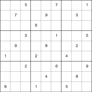
Then the solution is

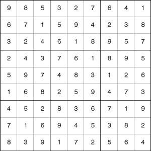
This solution can be found using the CLP procedure in SAS Optimization, with this code (note that the initial puzzle is entered in the step data indata and the final solution is nicely printed with the macro printSol).

data indata;
input C1-C9;
datalines;
. . 5 . . 7 . . 1
. 7 . . 9 . . 3 .
. . . 6 . . . . .
. . 3 . . 1 . . 5
. 9 . . 8 . . 2 .
1 . . 2 . . 4 . .
. . 2 . . 6 . . 9
. . . . 4 . . 8 .
8 . . 1 . . 5 . .
;
run;
%macro store_initial_values;
  /* store initial values into macro variable C_i_j */
  data _null_;
    set indata;
    array C{9};
    do j = 1 to 9;
      i = _N_;
      call symput(compress("C_" ||  put(i,best.)  || "_"  || put(j,best.)),
        put(C[j],best.));
    end;
  run;
 
%mend store_initial_values;
 
%store_initial_values;
 
%macro solve;
  proc clp out=outdata;
    %do i = 1 %to 9;
      var (X_&i._1-X_&i._9) = [1,9];
      alldiff(X_&i._1-X_&i._9);
    %end;
    %do j = 1 %to 9;
      alldiff(
        %do;
          i = 1 %to 9;
        X_&i._&j
        %end;
      );
    %end;
    %do s = 0 %to 2;
      %do t = 0 %to 2;
        alldiff(
          %do i = 3*&s + 1 %to 3*&s + 3;
            %do;
              j = 3*&t + 1 %to 3*&t + 3;
            X_&i._&j
            %end;
          %end;
          );
       %end;
     %end;
     %do i = 1 %to 9;
       %do j = 1 %to 9;
         %if &&C_&i._&j ne . %then
           %do;
             lincon X_&i._&j = &&C_&i._&j;
           %end;
       %end;
     %end;
    run;
 
    %put &_ORCLP_;
%mend solve;
 
%solve;
 
%macro printSol;
  data final (keep= A1 A2 A3 A4 A5 A6 A7 A8 A9);
    set outdata;
    array A{9};
    %do i = 1 %to 9;
      %do j = 1 %to 9;
        A(&j)=X_&i._&j;
      %end;
      output;
    %end;
  run;
 
%mend printSol;
 
%printSol;

Conclusion

Every optimization person could benefit from using Constraint programming. It is a powerful tool, which can be used in hybrid approaches with Integer Programming and heuristic procedures.

References

• SAS/OR® 22 User’s Guide: Constraint Programming
• Principles and Practice of Constraint Programming
• SAS® And Sudoku