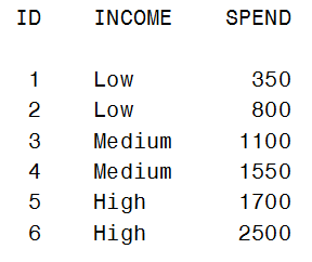
In the previous blog on CLASS variables, we developed the idea of creating design variables and examined GLM and reference coding. Another coding scheme, known as ‘Effect Coding’ or ‘Deviation from the Mean Coding’ is also commonly used. Consider our previous scenario of modeling the average amount spent on a credit card (SPEND) as a function of the variable INCOME (which has three levels: Low, Medium, and High). Here is the simple data set we’ll use:

Effect coding creates design variables by using -1s, 0s, and +1s. We replace the variable INCOME with two new design (or indicator) variables, ‘Low’ and ‘Medium’ as shown below:

data spend3;
  set spend1;
  Low=1*(income='Low')+0*(income='Medium')-1*(income='High');
  Medium=0*(income='Low')+1*(income='Medium')-1*(income='High');
run;

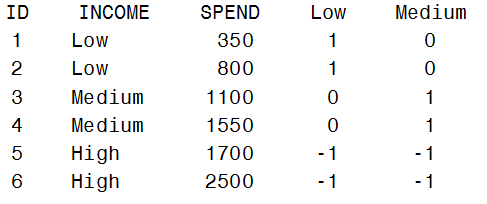
This is similar to reference coding, in that it uses only two design variables for the three-level INCOME variable. It differs in that the last level (High) is coded as -1 instead of 0. Recall that GLM coding creates three design variables and as a result “overparameterizes” the model.

When writing the PROC REG code for the model, use the design variables instead of the original variable INCOME; in the code below, High is the reference level because it is last on the MODEL statement:

proc reg data=spend3;
  model spend=low medium high;
run;

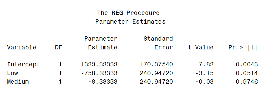
How do we interpret these parameters?  For effect coding, the intercept now represents the average amount spent in the population and is estimated to be 1333.3333. The parameter estimates for Low and Medium indicate how much above (for a positive parameter) or below (for a negative parameter) the SPEND amount is for observations in these categories, as compared to the average SPEND amount in the population.

The arithmetic gets a little messy due to the decimals, but for Low income, the SPEND amount is estimated to be:

1333.33333 - 758.33333 = 575

For Medium income, the estimated SPEND amount is:

1333.33333 - 8.33333 = 1325

To find the estimated SPEND amount for observations in the High category, look at the coding for the design variables for observations in that category:

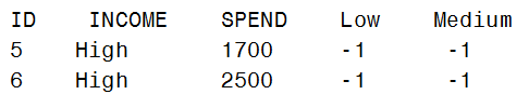
Notice that for these two observations the values of the indicator variables for Low and Medium are both -1. It may not be obvious, but to find the parameter for High, we take the negative of the parameter for Low and Medium and combine them:

-1*(-758.33333) -1*(8.33333) = 766.66666

This represents the deviation from the average. So the SPEND amount for High income is:

1333.33333 + 766.66666 = 2100 (rounding off)

To summarize, the average SPEND amounts are 575, 1325 and 2100 for income categories, Low, Medium, and High, respectively. While the parameter estimates are different than the ones obtained previously for GLM and reference coding, the estimated SPEND amounts are the same.

While we can always create our own design variables, several modeling procedures have a CLASS statement that will create them for us: GENMOD, GLM, GLIMMIX, LOGISTIC, MIXED, and others. Check the online documentation for each procedure to find what coding schemes and options are available for those pesky CLASS variables.