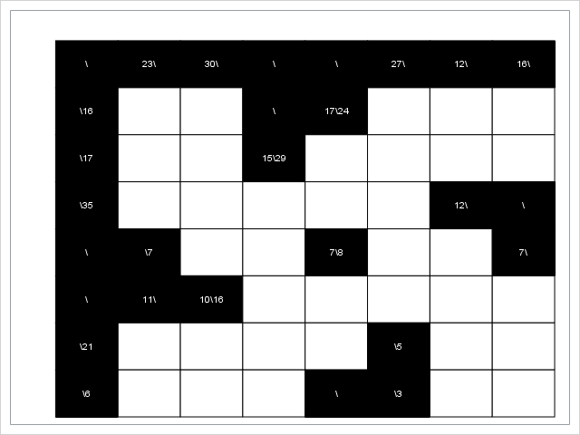
Erwin Kalvelagen recently posted about a logic puzzle called Kakuro, also known as Cross Sums. As in traditional crossword puzzles, there are horizontal and vertical clues. As in Sudoku, each white cell is to be filled in with a digit from 1 to 9, with no digit repeated within the same clue. Each number in a black cell indicates a required sum of digits; a number before the backslash is for the block of white cells immediately below, and a number after the backslash is for the block on the right.
For example, the 16 in the top left corner indicates that the first two white cells in the top row must add up to 16. Since they must also be distinct, the only two possibilities are 7 + 9 and 9 + 7.
Mixed Integer Linear Programming
The puzzle is of course meant to be solved by hand by making logical deductions. But you can also use mixed integer linear programming (MILP). One natural formulation involves two sets of decision variables:
For more details, see Kalvelagen's post.
You can capture the clues with a SAS data set:
%let n = 8; data indata; input (C1-C&n) ($); datalines; x\x 23\x 30\x x\x x\x 27\x 12\x 16\x x\16 x x x\x 17\24 x x x x\17 x x 15\29 x x x x x\35 x x x x x 12\x x\x x\x x\7 x x 7\8 x x 7\x x\x 11\x 10\16 x x x x x x\21 x x x x x\5 x x x\6 x x x x\x x\3 x x ; |
The following PROC OPTMODEL code declares sets and parameters, reads the data, declares the variables and constraints, calls the MILP solver, and outputs the solution to a SAS data set:
proc optmodel;
   set ROWS;
   set COLS = 1..&n;
   str clue {ROWS, COLS};

   /* read two-dimensional data */
   read data indata into ROWS=[_n_];
   read data indata into [i=_n_] {j in COLS} <clue[i,j] = col("c"||j)>;
   /* create output data set for use by PROC SGPLOT */
   create data puzzle from [i j]=(ROWS cross COLS)
      label=(compress(clue[i,j],'x')) color=(clue[i,j]='x');

   /* parse clues */
   num num_clues init 0;
   set CLUES = 1..num_clues;
   set <num,num> CELLS_c {CLUES} init {};
   num clue_length {c in CLUES} = card(CELLS_c[c]);
   num clue_sum {CLUES};
   str prefix, suffix;
   num curr;
   for {i in ROWS, j in COLS: clue[i,j] ne 'x'} do;
      prefix = scan(clue[i,j],1,'\');
      suffix = scan(clue[i,j],2,'\');
      if prefix ne 'x' then do;
         num_clues = num_clues + 1;
         clue_sum[num_clues] = input(prefix, best.);
         curr = i + 1;
         do until (curr not in ROWS or clue[curr,j] ne 'x');
            CELLS_c[num_clues] = CELLS_c[num_clues] union {<curr,j>};
            curr = curr + 1;
         end;
      end;
      if suffix ne 'x' then do;
         num_clues = num_clues + 1;
         clue_sum[num_clues] = input(suffix, best.);
         curr = j + 1;
         do until (curr not in COLS or clue[i,curr] ne 'x');
            CELLS_c[num_clues] = CELLS_c[num_clues] union {<i,curr>};
            curr = curr + 1;
         end;
      end;
   end;
   set CELLS = union {c in CLUES} CELLS_c[c];
   set DIGITS = 1..9;

   /* decision variables */
   var X {CELLS, DIGITS} binary;
   var V {CELLS} integer >= 1 <= 9;

   /* constraints */
   con OneDigitPerCell {<i,j> in CELLS}:
      sum {k in DIGITS} X[i,j,k] = 1;

   con AlldiffPerClue {c in CLUES, k in DIGITS}:
      sum {<i,j> in CELLS_c[c]} X[i,j,k] <= 1;

   con VCon {<i,j> in CELLS}:
      sum {k in DIGITS} k * X[i,j,k] = V[i,j];

   con SumCon {c in CLUES}:
      sum {<i,j> in CELLS_c[c]} V[i,j] = clue_sum[c];

   /* call MILP solver with no objective */
   solve noobj;

   /* create output data set for use by PROC SGPLOT */
   create data solution from [i j]=(ROWS cross COLS) V
      label=(if <i,j> in CELLS then put(V[i,j],1.) else compress(clue[i,j],'x')) color=(<i,j> in CELLS);
quit; |
Notice that the PROC OPTMODEL code is completely data-driven so that you can solve other problem instances just by changing the input data set. In this case, the MILP presolver solves the entire problem instantly:
NOTE: Problem generation will use 4 threads.
NOTE: The problem has 360 variables (0 free, 0 fixed).
NOTE: The problem has 324 binary and 36 integer variables.
NOTE: The problem has 312 linear constraints (216 LE, 96 EQ, 0 GE, 0 range).
NOTE: The problem has 1404 linear constraint coefficients.
NOTE: The problem has 0 nonlinear constraints (0 LE, 0 EQ, 0 GE, 0 range).
NOTE: The OPTMODEL presolver is disabled for linear problems.
NOTE: The MILP presolver value AUTOMATIC is applied.
NOTE: The MILP presolver removed all variables and constraints.
NOTE: Optimal.
NOTE: Objective = 0.
Finally, a call to PROC SGPLOT generates a nice plot of the solution:
proc sgplot data=solution noautolegend; heatmapparm x=j y=i colorresponse=color / colormodel=(black white) outline; text x=j y=i text=label / colorresponse=color colormodel=(white black); xaxis display=none; yaxis display=none reverse; run; |
The resulting plot makes it easy to verify the correctness of the solution:

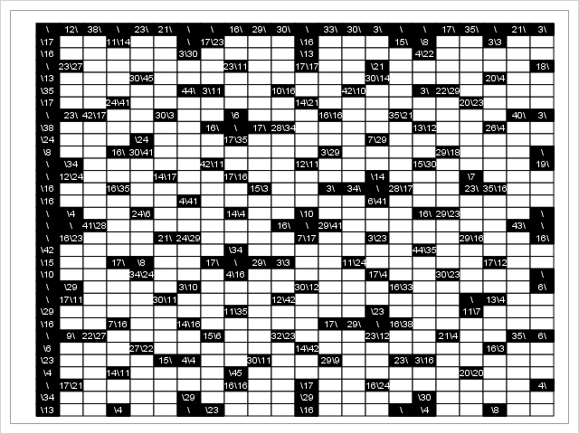
Here is the corresponding DATA step for the large instance in Kalvelagen's post:
%let n = 22; data indata; input (C1-C&n) ($); datalines; x\x 12\x 38\x x\x 23\x 21\x x\x x\x 16\x 29\x 30\x x\x 33\x 30\x 3\x x\x x\x 17\x 35\x x\x 21\x 3\x x\17 x x 11\14 x x x\x 17\23 x x x x\16 x x x 15\x x\8 x x 3\3 x x x\16 x x x x x 3\30 x x x x x\13 x x x x 4\22 x x x x x x\x 23\27 x x x x x x 23\11 x x 17\17 x x x\21 x x x x x x 18\x x\13 x x x 30\45 x x x x x x x x x 30\14 x x x x 20\4 x x x\35 x x x x x 44\x 3\11 x x 10\16 x x 42\10 x x 3\x 22\29 x x x x x\17 x x 24\41 x x x x x x x 14\21 x x x x x x 20\23 x x x x\x 23\x 42\17 x x 30\3 x x x\6 x x x 16\16 x x 35\21 x x x x 40\x 3\x x\38 x x x x x x 16\x x\x 17\x 28\34 x x x x x 13\12 x x 26\4 x x x\24 x x x x\24 x x x 17\35 x x x x x 7\29 x x x x x x x x\8 x x 16\x 30\41 x x x x x x x 3\29 x x x x 29\18 x x x x\x x\x x\34 x x x x x 42\11 x x x 12\11 x x x x 15\30 x x x x 19\x x\x 12\24 x x x 14\17 x x 17\16 x x x x x x\14 x x x x\7 x x x x\16 x x 16\35 x x x x x 15\3 x x 3\x 34\x x\x 28\17 x x 23\x 35\16 x x x\16 x x x x x 4\41 x x x x x x x 6\41 x x x x x x x x\x x\4 x x 24\6 x x x 14\4 x x x\10 x x x x 16\x 29\23 x x x x\x x\x x\x 41\28 x x x x x x x 16\x x\x 29\41 x x x x x x x 43\x x\x x\x 16\23 x x x 21\x 24\29 x x x x 7\17 x x 3\23 x x x 29\16 x x 16\x x\42 x x x x x x x x\34 x x x x x x x 44\35 x x x x x x\15 x x 17\x x\8 x x 17\x x\x 29\x 3\3 x x 11\24 x x x x x 17\12 x x x\10 x x x 34\24 x x x 4\16 x x x x x 17\4 x x 30\23 x x x x\x x\x x\29 x x x x 3\10 x x x x 30\12 x x x 16\33 x x x x x 6\x x\x 17\11 x x x 30\11 x x x x 12\42 x x x x x x x x\x 13\4 x x x\29 x x x x x x x 11\35 x x x x x x\23 x x x 11\7 x x x x\16 x x 7\16 x x 14\16 x x x x x 17\x 29\x x\x 16\38 x x x x x x x\x 9\x 22\27 x x x x 15\6 x x 32\23 x x x 23\12 x x 21\4 x x 35\x 6\x x\6 x x x 27\22 x x x x x x 14\42 x x x x x x x 16\3 x x x\23 x x x x 15\x 4\4 x x 30\11 x x 29\9 x x 23\x 3\16 x x x x x x\4 x x 14\11 x x x x x\45 x x x x x x x x x 20\20 x x x x\x 17\21 x x x x x x 16\16 x x x\17 x x 16\24 x x x x x x 4\x x\34 x x x x x x\29 x x x x x\29 x x x x x\30 x x x x x x\13 x x x\4 x x x\x x\23 x x x x\16 x x x x\x x\4 x x x\8 x x ; |
And here is the plot of the input:

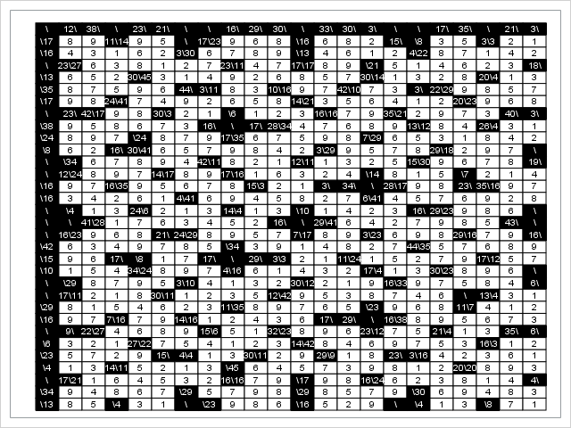
The same PROC OPTMODEL and PROC SGPLOT statements shown earlier then yield the following output:
NOTE: Problem generation will use 4 threads.
NOTE: The problem has 4920 variables (0 free, 0 fixed).
NOTE: The problem has 4428 binary and 492 integer variables.
NOTE: The problem has 3664 linear constraints (2412 LE, 1252 EQ, 0 GE, 0 range).
NOTE: The problem has 19188 linear constraint coefficients.
NOTE: The problem has 0 nonlinear constraints (0 LE, 0 EQ, 0 GE, 0 range).
NOTE: The OPTMODEL presolver is disabled for linear problems.
NOTE: The MILP presolver value AUTOMATIC is applied.
NOTE: The MILP presolver removed 3077 variables and 2087 constraints.
NOTE: The MILP presolver removed 12000 constraint coefficients.
NOTE: The MILP presolver added 22 constraint coefficients.
NOTE: The MILP presolver modified 11 constraint coefficients.
NOTE: The presolved problem has 1843 variables, 1577 constraints, and 7188 constraint
      coefficients.
NOTE: The MILP solver is called.
NOTE: The parallel Branch and Cut algorithm is used.
NOTE: The Branch and Cut algorithm is using up to 4 threads.
          Node  Active    Sols    BestInteger      BestBound      Gap    Time
             0       1       0              .              0        .       2
NOTE: The MILP presolver is applied again.
             0       0       1              0              0    0.00%       2
NOTE: Optimal.
NOTE: Objective = 0.
Constraint Programming
Default Settings
The requirement that the digits within a single clue must all be different suggests the use of the ALLDIFF constraint supported in the constraint programming solver. You can then omit the binary X[i,j,k] variables and the corresponding constraints. The resulting model is much simpler, with only one set of variables and two sets of constraints:
/* decision variables */ var V {CELLS} integer >= 1 <= 9; /* constraints */ con AlldiffCon {c in CLUES}: alldiff({<i,j> in CELLS_c[c]} V[i,j]); con SumCon {c in CLUES}: sum {<i,j> in CELLS_c[c]} V[i,j] = clue_sum[c]; /* call constraint programming solver */ solve; |
For the small instance, the constraint programming solver instantly returns the solution:
NOTE: Problem generation will use 4 threads.
NOTE: The problem has 36 variables (0 free, 0 fixed).
NOTE: The problem has 0 binary and 36 integer variables.
NOTE: The problem has 24 linear constraints (0 LE, 24 EQ, 0 GE, 0 range).
NOTE: The problem has 72 linear constraint coefficients.
NOTE: The problem has 0 nonlinear constraints (0 LE, 0 EQ, 0 GE, 0 range).
NOTE: The problem has 24 predicate constraints.
NOTE: The OPTMODEL presolver is disabled for problems with predicates.
NOTE: Required number of solutions found (1).
NOTE: The data set WORK.SOLUTION has 64 observations and 5 variables.
NOTE: PROCEDURE OPTMODEL used (Total process time):
      real time           0.10 seconds
      cpu time            0.06 seconds
Precomputation of Domain Reduction
But the large instance is more challenging and does not solve in a reasonable time, for reasons described in a paper by Helmut Simonis. One way to overcome this difficulty is to first do some precomputation, again with the constraint programming solver, to prune the domains of the decision variables. The idea is to consider each clue one at a time, using the FINDALLSOLNS option to find all solutions. Any digit that does not appear among these solutions can then be removed, by using a linear disequality (or "not equal") constraint, from the domains of the V[i,j] variables that are associated with that clue. Because these problems are independent across clues, you can use a COFOR loop to solve them concurrently. The full code is as follows:
proc optmodel;
   set ROWS;
   set COLS = 1..&n;
   str clue {ROWS, COLS};

   /* read two-dimensional data */
   read data indata into ROWS=[_n_];
   read data indata into [i=_n_] {j in COLS} <clue[i,j] = col("c"||j)>;
   /* create output data set for use by PROC SGPLOT */
   create data puzzle from [i j]=(ROWS cross COLS)
      label=(compress(clue[i,j],'x')) color=(clue[i,j]='x');

   /* parse clues */
   num num_clues init 0;
   set CLUES = 1..num_clues;
   set <num,num> CELLS_c {CLUES} init {};
   num clue_length {c in CLUES} = card(CELLS_c[c]);
   num clue_sum {CLUES};
   str prefix, suffix;
   num curr;
   for {i in ROWS, j in COLS: clue[i,j] ne 'x'} do;
      prefix = scan(clue[i,j],1,'\');
      suffix = scan(clue[i,j],2,'\');
      if prefix ne 'x' then do;
         num_clues = num_clues + 1;
         clue_sum[num_clues] = input(prefix, best.);
         curr = i + 1;
         do until (curr not in ROWS or clue[curr,j] ne 'x');
            CELLS_c[num_clues] = CELLS_c[num_clues] union {<curr,j>};
            curr = curr + 1;
         end;
      end;
      if suffix ne 'x' then do;
         num_clues = num_clues + 1;
         clue_sum[num_clues] = input(suffix, best.);
         curr = j + 1;
         do until (curr not in COLS or clue[i,curr] ne 'x');
            CELLS_c[num_clues] = CELLS_c[num_clues] union {<i,curr>};
            curr = curr + 1;
         end;
      end;
   end;
   set CELLS = union {c in CLUES} CELLS_c[c];
   set DIGITS = 1..9;

   /* decision variables */
   var V {CELLS} integer >= 1 <= 9;

   /* constraints */
   con AlldiffCon {c in CLUES}:
      alldiff({<i,j> in CELLS_c[c]} V[i,j]);

   con SumCon {c in CLUES}:
      sum {<i,j> in CELLS_c[c]} V[i,j] = clue_sum[c];

   problem Original include
      V AlldiffCon SumCon;

   /* prune the domains one clue at a time */
   set DOMAIN {CELLS};
   set LENGTHS_SUMS = setof {c in CLUES} <clue_length[c], clue_sum[c]>;
   set DOMAIN_ls {LENGTHS_SUMS};
   num clue_length_this, clue_sum_this;
   var W {1..clue_length_this} integer >= 1 <= 9;
   con IncreasingWCon {k in 1..clue_length_this-1}:
      W[k] < W[k+1];
   con SumWCon {c in CLUES}:
      sum {k in 1..clue_length_this} W[k] = clue_sum_this;
   problem Prune include
      W IncreasingWCon SumWCon;
   use problem Prune;
   reset options printlevel=0;
   cofor {<l,s> in LENGTHS_SUMS} do;
      put l= s=;
      clue_length_this = l;
      clue_sum_this    = s;
      solve with clp / findallsolns;
      DOMAIN_ls[l,s] = setof {k in 1..clue_length_this, sol in 1.._NSOL_} W[k].sol[sol];
      put DOMAIN_ls[l,s]=;
   end;
   reset options printlevel;
   for {<i,j> in CELLS} DOMAIN[i,j] = DIGITS;
   for {c in CLUES} do;
      clue_length_this = clue_length[c];
      clue_sum_this    = clue_sum[c];
      for {<i,j> in CELLS_c[c]}
         DOMAIN[i,j] = DOMAIN[i,j] inter DOMAIN_ls[clue_length_this, clue_sum_this];
   end;
   for {<i,j> in CELLS} put DOMAIN[i,j]=;

   /* solve original problem with pruned domains */
   use problem Original;
   con PruneDomain {<i,j> in CELLS, k in DIGITS diff DOMAIN[i,j]}:
      V[i,j] ne k;
   solve;

   /* create output data set for use by PROC SGPLOT */
   create data solution from [i j]=(ROWS cross COLS) V
      label=(if <i,j> in CELLS then put(V[i,j],1.) else compress(clue[i,j],'x')) color=(<i,j> in CELLS);
quit; |
The entire PROC OPTMODEL call, including the precomputation step, now takes less than a second for the large instance:
NOTE: Problem generation will use 4 threads.
NOTE: The problem has 492 variables (0 free, 0 fixed).
NOTE: The problem has 0 binary and 492 integer variables.
NOTE: The problem has 2878 linear constraints (0 LE, 268 EQ, 0 GE, 0 LT, 2610 NE, 0 GT, 0
      range).
NOTE: The problem has 3594 linear constraint coefficients.
NOTE: The problem has 0 nonlinear constraints (0 LE, 0 EQ, 0 GE, 0 range).
NOTE: The problem has 268 predicate constraints.
NOTE: The OPTMODEL presolver is disabled for problems with predicates.
NOTE: Required number of solutions found (1).
NOTE: The data set WORK.SOLUTION has 704 observations and 5 variables.
NOTE: PROCEDURE OPTMODEL used (Total process time):
      real time           0.53 seconds
      cpu time            0.96 seconds
VARSELECT= Option
It turns out that you can also significantly improve the performance without doing any precomputation, simply by using a different variable selection strategy:
solve with clp / varselect=fifo; |
NOTE: Problem generation will use 4 threads.
NOTE: The problem has 492 variables (0 free, 0 fixed).
NOTE: The problem has 0 binary and 492 integer variables.
NOTE: The problem has 268 linear constraints (0 LE, 268 EQ, 0 GE, 0 range).
NOTE: The problem has 984 linear constraint coefficients.
NOTE: The problem has 0 nonlinear constraints (0 LE, 0 EQ, 0 GE, 0 range).
NOTE: The problem has 268 predicate constraints.
NOTE: Required number of solutions found (1).
NOTE: The data set WORK.SOLUTION has 704 observations and 5 variables.
NOTE: PROCEDURE OPTMODEL used (Total process time):
      real time           6.55 seconds
      cpu time            6.42 seconds
Checking Uniqueness
As in similar logic puzzles, the solution is supposed to be unique. To check uniqueness with the MILP formulation, you can add one more constraint to exclude the first solution and call the MILP solver again, as described by Kalvelagen:
/* check uniqueness */ set <num,num,num> SUPPORT; SUPPORT = {<i,j> in CELLS, k in DIGITS: X[i,j,k].sol > 0.5}; con ExcludeSolution: sum {<i,j,k> in SUPPORT} X[i,j,k] <= card(SUPPORT) - 1; solve noobj; if _solution_status_ ne 'INFEASIBLE' then put 'Multiple solutions found!'; |
For the constraint programming formulation, checking uniqueness is even simpler. Just use the FINDALLSOLNS option:
/* check uniqueness */ solve with clp / findallsolns; if _NSOL_ > 1 then put 'Multiple solutions found!'; |

