This article implements Passing-Bablok regression in SAS. Passing-Bablok regression is a one-variable regression technique that is used to compare measurements from different instruments or medical devices. The measurements of the two variables (X and Y) are both measured with errors. Consequently, you cannot use ordinary linear regression, which assumes that one variable (X) is measured without error. Passing-Bablok regression is a robust nonparametric regression method that does not make assumptions about the distribution of the expected values or the error terms in the model. It also does not assume that the errors are homoscedastic.
Several readers have asked about Passing-Bablok regression because I wrote an article about Deming regression, which is similar. On the SAS Support Communities, there was a lively discussion in response to a program by KSharp in which he shows how to use Base SAS procedures to perform a Passing-Bablok regression. In response to this interest, this article shares a SAS/IML program that performs Passing-Bablok regression.
An overview of Passing-Bablok regression
Passing-Bablok regression (Passing and Bablok, 1983, J. Clin. Chem. Clin. Biochem., henceforth denote PB) fits a line through X and Y measurements. The X and Y variables measure the same quantity in the same units. Usually, X is the "gold standard" technique, whereas Y is a new method that is cheaper, more accurate, less invasive, or has some other favorable attributes. Whereas Deming regression assumes normal errors, Passing-Bablok regression can handle any error distribution provided that the measurement errors for both methods follow the same distribution. Also, the variance of each method does not need to be constant across the range of data. All that is required is that the ratio of the variances is constant. The Passing-Bablok method is robust to outliers in X or Y.
Assume you have N pairs of observations {(xi, yi), i=1..N}, where X and Y are different ways to measure the same quantity. Passing-Bablok regression determines whether the measurements methods are equivalent by estimating a line y = a + b*x. The estimate of the slope (b) is based on the median of pairs of slopes Sij = (yi - yj) / (xi - xj) for i < j. You must be careful when xi=xj. PB suggest assigning a large positive value when xi=xj and yi > yj and a large negative value when xi=xj and yi < yj. If xi=xj and yi=yj, the difference is not computed or used.
The Passing-Bablok method estimates the regression line y = a + b*x by using the following steps:- Compute all the pairwise slopes. For vertical slopes, use large positive or negative values, as appropriate.
- Exclude slopes that are exactly -1. The reason is technical, but it involves ensuring the same conclusions whether you regress Y onto X or X onto Y.
- Ideally, we would estimate the slope of the regression line (b) as the median of all the pairwise slopes of the points (xi, yi) and (xj, yj), where i < j. This is a robust statistic and is similar to Theil-Sen regression. However, the slopes are not independent, so the median can be a biased estimator. Instead, estimate the slope as the shifted median of the pairwise slopes.
- Estimate the intercept, a, as the median of the values {yi – bxi}.
- Use a combination of symmetry, rank-order statistics, and asymptotics to obtain confidence intervals (CIs) for b and a.
- You can use the confidence intervals (CIs) to assess whether the two methods are equivalent. In terms of the regression estimates, the CI for the intercept (a) must contain 0 and the CI for the slope (b) must contain 1. This article uses only the CIs proposed by Passing and Bablok. Some software support jackknife or bootstrap CIs, but it is sometimes a bad idea to use resampling methods to estimate the CI of a median, so I do not recommend bootstrap CIs for Passing-Bablok regression.
Implement Passing-Bablok regression in SAS
Because the Passing-Bablok method relies on computing vectors and medians, the SAS/IML language is a natural language for implementing the algorithm. The implementation uses several helper functions from previous articles:
- The StrictLowerTriangular function extracts the elements below the diagonal in a square matrix.
- The PairwiseDiff function returns all pairwise differences in a vector of values.
The following modules implement the Passing-Bablok algorithm in SAS and store the modules for future use:
%let INFTY = 1E12; /* define a big number to use as "infinity" for vertical slopes */ proc iml; /* Extract only the values X[i,j] where i < j. https://blogs.sas.com/content/iml/2012/08/16/extract-the-lower-triangular-elements-of-a-matrix.html */ start StrictLowerTriangular(X); v = cusum( 1 || (ncol(X):2) ); return( remove(vech(X), v) ); finish; /* Compute pairwise differences: https://blogs.sas.com/content/iml/2011/02/09/computing-pairwise-differences-efficiently-of-course.html */ start PairwiseDiff(x); /* x is a column vector */ n = nrow(x); m = shape(x, n, n); /* duplicate data */ diff = m` - m; /* pairwise differences */ return( StrictLowerTriangular(diff) ); finish; /* Implement the Passing-Bablok (1983) regression method */ start PassingBablok(_x, _y, alpha=0.05, debug=0); keepIdx = loc(_x^=. & _y^=.); /* 1. remove missing values */ x = _x[keepIdx]; y = _y[keepIdx]; nObs = nrow(x); /* sample size of nonmissing values */ /* 1. Compute all the pairwise slopes. For vertical, use large positive or negative values. */ DX = T(PairwiseDiff(x)); /* x[i] - x[j] */ DY = T(PairwiseDiff(y)); /* y[i] - y[j] */ /* "Identical pairs of measurements with x_i=x_j and y_i=y_j do not contribute to the estimation of beta." (PB, p 711) */ idx = loc(DX^=0 | DY^=0); /* exclude 0/0 slopes (DX=0 and DY=0) */ G = DX[idx] || DY[idx] || j(ncol(idx), 1, .); /* last col is DY/DX */ idx = loc( G[,1] ^= 0 ); /* find where DX ^= 0 */ G[idx,3] = G[idx,2] / G[idx,1]; /* form Sij = DY / DX for DX^=0 */ /* Special cases: 1) x_i=x_j, but y_i^=y_j ==> Sij = +/- infinity 2) x_i^=x_j, but y_i=y_j ==> Sij = 0 "The occurrence of any of these special cases has a probability of zero (experimental data should exhibit these cases very rarely)." Passing and Bablok do not specify how to handle, but one way is to keep these values within the set of valid slopes. Use large positive or negative numbers for +infty and -infty, respectively. */ posIdx = loc(G[,1]=0 & G[,2]>0); /* DX=0 & DY>0 */ if ncol(posIdx) then G[posIdx,3] = &INFTY; negIdx = loc(G[,1]=0 & G[,2]<0); /* DX=0 & DY<0 */ if ncol(negIdx) then G[negIdx,3] = -&INFTY; if debug then PRINT (T(1:nrow(G)) || G)[c={"N" "DX" "DY" "S"}]; /* 2. Exclude slopes that are exactly -1 */ /* We want to be able to interchange the X and Y variables. "For reasons of symmetry, any Sij with a value of -1 is also discarded." */ idx = loc(G[,3] ^= -1); S = G[idx,3]; N = nrow(S); /* number of valid slopes */ call sort(S); /* sort slopes ==> pctl computations easier */ if debug then print (S`)[L='sort(S)']; /* 3. Estimate the slope as the shifted median of the pairwise slopes. */ K = sum(S < -1); /* shift median by K values */ b = choose(mod(N,2), /* estimate of slope */ S[(N+1)/2+K ], /* if N odd, shifted median */ mean(S[N/2+K+{0,1}])); /* if N even, average of adjacent values */ /* 4. Estimate the intercept as the median of the values {yi – bxi}. */ a = median(y - b*x); /* estimate of the intercept, a */ /* 5. Estimate confidence intervals. */ C = quantile("Normal", 1-alpha/2) * sqrt(nObs*(nObs-1)*(2*nObs+5)/18); M1 = round((N - C)/2); M2 = N - M1 + 1; if debug then PRINT K C M1 M2 (M1+K)[L="M1+K"] (M2+k)[L="M1+K"]; CI_b = {. .}; /* initialize CI to missing */ if 1 <= M1+K & M1+K <= N then CI_b[1] = S[M1+K]; if 1 <= M2+K & M2+K <= N then CI_b[2] = S[M2+K]; CI_a = median(y - CI_b[,2:1]@x); /* aL=med(y-bU*x); aU=med(y-bL*x); */ /* return a list that contains the results */ outList = [#'a'=a, #'b'=b, #'CI_a'=CI_a, #'CI_b'=CI_b]; /* pack into list */ return( outList ); finish; store module=(StrictLowerTriangular PairwiseDiff PassingBablok); quit; |
Notice that the PassingBablok function returns a list. A list is a convenient way to return multiple statistics from a function.
Perform Passing-Bablok regression in SAS
Having saved the SAS/IML modules, let's see how to call the PassingBablok routine and analyze the results. The following DATA step defines 102 pairs of observations. These data were posted to the SAS Support Communities by @soulmate. To support running regressions on multiple data sets, I use macro variables to store the name of the data set and the variable names.
data PBData; label x="Method 1" y="Method 2"; input x y @@; datalines; 0.07 0.07 0.04 0.10 0.07 0.08 0.05 0.10 0.06 0.08 0.06 0.07 0.03 0.05 0.04 0.05 0.05 0.08 0.05 0.10 0.12 0.21 0.10 0.17 0.03 0.11 0.18 0.24 0.29 0.33 0.05 0.05 0.04 0.05 0.11 0.21 0.38 0.36 0.04 0.05 0.03 0.06 0.06 0.07 0.46 0.27 0.08 0.05 0.02 0.09 0.12 0.23 0.16 0.25 0.07 0.10 0.07 0.07 0.04 0.06 0.11 0.23 0.23 0.21 0.15 0.20 0.05 0.07 0.04 0.14 0.05 0.11 0.17 0.26 8.43 8.12 1.86 1.47 0.17 0.27 8.29 7.71 5.98 5.26 0.57 0.43 0.07 0.10 0.06 0.11 0.21 0.24 8.29 7.84 0.28 0.23 8.25 7.79 0.18 0.25 0.17 0.22 0.15 0.21 8.33 7.67 5.58 5.05 0.09 0.14 1.00 3.72 0.09 0.13 3.88 3.54 0.51 0.42 4.09 3.64 0.89 0.71 5.61 5.18 4.52 4.15 0.09 0.12 0.05 0.05 0.05 0.05 0.04 0.07 0.05 0.07 0.09 0.11 0.03 0.05 2.27 2.08 1.50 1.21 5.05 4.46 0.22 0.25 2.13 1.93 0.05 0.08 4.09 3.61 1.46 1.13 1.20 0.97 0.02 0.05 1.00 1.00 3.39 3.11 1.00 0.05 2.07 1.83 6.68 6.06 3.00 2.97 0.06 0.09 7.17 6.55 1.00 1.00 2.00 0.05 2.91 2.45 3.92 3.36 1.00 1.00 7.20 6.88 6.42 5.83 2.38 2.04 1.97 1.76 4.72 4.37 1.64 1.25 5.48 4.77 5.54 5.16 0.02 0.06 ; %let DSName = PBData; /* name of data set */ %let XVar = x; /* name of X variable (Method 1) */ %let YVar = y; /* name of Y variable (Method 2) */ title "Measurements from Two Methods"; proc sgplot data=&DSName noautolegend; scatter x=&XVar y=&YVar; lineparm x=0 y=0 slope=1 / clip; /* identity line: Intercept=0, Slope=1 */ xaxis grid; yaxis grid; run; |
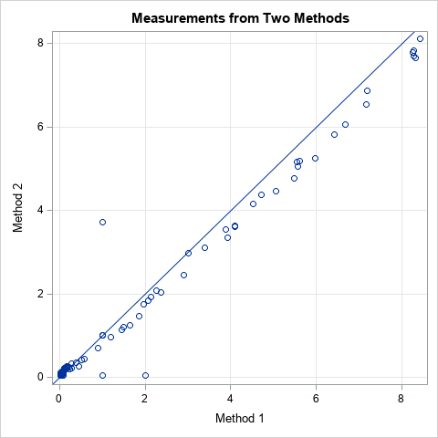
The graph indicates that the two measurements are linearly related and strongly correlated. It looks like Method 1 (X) produces higher measurements than Method 2 (Y) because most points are to the right of the identity line. Three outliers are visible. The Passing-Bablok regression should be robust to these outliers.
The following SAS/IML program analyzes the data by calling the PassingBablok function:
proc iml; load module=(StrictLowerTriangular PairwiseDiff PassingBablok); use &DSName; read all var {"&XVar"} into x; read all var {"&YVar"} into y; close; R = PassingBablok(x, y); ParameterEstimates = (R$'a' || R$'CI_a') // /* create table from the list items */ (R$'b' || R$'CI_b'); print ParameterEstimates[c={'Estimate' 'LCL' 'UCL'} r={'Intercept' 'Slope'}]; |
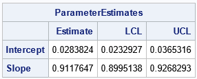
The program reads the X and Y variables and calls the PassingBablok function, which returns a list of statistics. You can use the ListPrint subroutine to print the items in the list, or you can extract the items and put them into a matrix, as in the example.
The output shows that the Passing-Bablok regression line is Y = 0.028 + 0.912*X. The confidence interval for the slope parameter (b) does NOT include 1, which means that we reject the null hypothesis that the measurements are related by a line that has unit slope. Even if the CI for the slope had contained 1, the CI for the Intercept (a) does not include 0. For these data, we reject the hypothesis that the measurements from the two methods are equivalent.
Of course, you could encapsulate the program into a SAS macro that performs Passing-Bablok regression.
A second example of Passing-Bablok regression in SAS
For completeness, the following example shows results for two methods that are equivalent. The output shows that the CI for the slope includes 1 and the CI for the intercept includes 0:
%let DSName = PBData2; /* name of data set */ %let XVar = m1; /* name of X variable (Method 1) */ %let YVar = m2; /* name of Y variable (Method 2) */ data &DSName; label m1="Method 1" m2="Method 2"; input m1 m2 @@; datalines; 10.1 10.1 10.5 10.6 12.8 13.1 8.7 8.7 10.8 11.5 10.6 10.4 9.6 9.9 11.3 11.3 7.7 7.5 11.5 11.9 7.9 7.8 9.9 9.7 9.3 9.9 16.3 16.2 9.4 9.8 11.0 11.8 9.1 8.7 12.2 11.9 13.4 12.6 9.2 9.5 8.8 9.1 9.3 9.2 8.5 8.7 9.6 9.7 13.5 13.1 9.4 9.1 9.5 9.6 10.8 11.3 14.6 14.8 9.7 9.3 16.4 16.5 8.1 8.6 8.3 8.1 9.5 9.6 20.3 20.4 8.6 8.5 9.1 8.8 8.8 8.7 9.2 9.9 8.1 8.1 9.2 9.0 17.0 17.0 10.2 10.0 10.0 9.8 6.5 6.6 7.9 7.6 11.3 10.7 14.2 14.1 11.9 12.7 9.9 9.4 ; proc iml; load module=(StrictLowerTriangular PairwiseDiff PassingBablok); use &DSName; read all var {"&XVar"} into x; read all var {"&YVar"} into y; close; R = PassingBablok(x, y); ParameterEstimates = (R$'a' || R$'CI_a') // (R$'b' || R$'CI_b'); print ParameterEstimates[c={'Estimate' 'LCL' 'UCL'} r={'Intercept' 'Slope'}]; QUIT; |
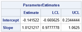
For these data, the Passing-Bablok regression line is Y = -0.142 + 1.012*X. The confidence interval for the Slope term is [0.98, 1.06], which contains 1. The confidence interval for the Intercept is [-0.67, 0.23], which contains 0. Thus, these data suggest that the two methods are equivalent ways to measure the same quantity.
Summary
This article shows how to implement Passing-Bablok regression in SAS by using the SAS/IML language. It also explains how Passing-Bablok regression works and why different software might provide different confidence intervals. You can download the complete SAS program that implements Passing-Bablok regression and creates the graphs and tables in this article.
Further Reading
- "An example of Passing-Bablok Regression in SAS" by KSharp is a program that uses only Base SAS procedures. He also includes a PDF of the Passing-Bablok paper.
- "Passing-Bablok Regression: R code for SAS users" by Clint Stevenson. Includes a discussion of why the default regression in the mcr package in R is different from method in the Passing-Bablok paper.
- Documentation of the Passing-Bablok regression in the NCSS software package.
- The mcr package in R by Manuilova, Schuetzenmeister, and Model contains several regression methods for method-comparison regression.
Appendix: Comparing the results of Passing-Bablok regression
The PB paper is slightly ambiguous about how to handle certain special situations in the data. The ambiguity is in the calculation of confidence intervals. Consequently, if you run the same data through different software, you are likely to obtain the same point estimates, but the confidence intervals might be slightly different (maybe in the third or fourth decimal place), especially when there are repeated X values that have multiple Y values. For example, I have compared my implementation to MedCalc software and to the mcr package in R. The authors of the mcr package made some choices that are different from the PB paper. By looking at the code, I can see that they handle tied data values differently from the way I handle them.

16 Comments
Rick,
Finally see this blog from you . I will tested it by Medcalc .
Good Job !
Rick,
In your second example.
label x="Method 1" y="Method 2";
should be
label m1="Method 1" m2="Method 2";
?
Thanks.
Rick,
It looks like you do not calculate bootstrap CI ?
Could you include it in your blog ?
Thanks for the comment. Since PB regression is a robust and distribution-free method, there is no reason to resort to bootstrap methods. In the article, I mention why I do not recommend bootstrap CIs. Furthermore, I haven't seen any examples where a bootstrap gives substantially different CIs from the PB estimates.
Hi Rick,
For The Passing-Bablok regression, there are 2 more questions.
question 1:
Although Passing-Bablok regression requires very little of a variable distribution, it also has its own hypothesis, namely the Cuban test for linearity. I read from some literature, if linearity test failed, Passing-Bablok regression should not be uesd.
How do you think about this? Should the corresponding hypothesis test be included in the program?
question 2:
For the bootstrap CI problem, I've also read from some literature that they suggest using this technique for PB regression.
Take EP09-A3 as an example, it explicitly suggests that PB regression should use the bootstrap method for CI estimation. However, it is not recommended to use the jackknife method for ci estimation. And it gives an example in Appendix I as to why the bootstrap method is appropriate and more real.
In your other articles on examples of the application of the bootstrap method, you concluded that the bootstrap method is not a good way to estimate CI. But for nonparametric PB regression, the sample size is usually not enough to estimate an accurate CI, and this problem can only be solved by the bootstrap method, right?
And for the skewed data, the distribution obtained by the bootstrap sampling method is necessarily not normal, and it is also possible to amplify the bias of the original data (such as 30 in your example, which is more pumped) to make the data look more skewed.
So for bootstrap estimation CI, I personally think it is still necessary. What do you think? Can you explain it more easily?
thanks!
1. Yes, the data should be linearly related if you are going to apply a linear regression model. You can graph the data to see if they are linearly related, or you can run a more formal hypothesis test. Passing and Bablok suggest a CUSUM test for perpendicular distances to the regression line. Thus, you have to compute the regression estimates (a,b) first, and the test is conditional on the estimates.
2. You are free to use a bootstrap CI if that makes you happy. I have not read EP09-A3, so I cannot comment on it. I do not know who wrote it or the theoretical basis for their recommendations.
PB discuss the CIs in Appendix 3. An assumption is that a certain quantity (which they call C) is normally distributed. You can prove that C is asymptotically normal, so for large data, the CIs are valid. PB did a simulation study for samples of size 40 <= n <= 60 and reported that "in all cases the actual confidence level is about 95%; it is never less than 91% or higher than 96%" (p. 719). They do not provide any information about samples with fewer than 40 observations. However, they note that "the actual level of the confidence interval for alpha is higher than 95%."
I can tell you that a bootstrap sample contains duplicate values for some pairs and omits other pairs. On average, a bootstrap sample omits 36.8% of the data, which means that you get a lot of duplicates. In the PB regression, "identical pairs of measurements with x_i=x_j and y_i=y_j do not contribute to the estimation of beta" (p. 711). The PB regression method excludes these duplicate values. Consequently, the average bootstrap sample discards 37% of the data. Thus, I would expect a bootstrap CI to be wider than necessary. Wide CIs means that you would accept the hypothesis that the measurement methods are equivalent more often than you should. Until someone shows me an argument that changes my mind, I do not recommend boostrap CIs.
Dear Rick,
Thank you for this very nice introduction into Passing-Bablok regression and a possible implementation in SAS!
Like the late Wolfgang Bablok, I work at Roche Diagnostics, Germany. Therefore, the use and discussion of Passing-Bablok regression has a strong tradition in our company. Some of the insights gained since have recently been published (see below).
But let me first make some remarks on the bootstrap estimator for the CIs of the slope:
The effect of the duplicate values on the bootstrap estimator of the variance or CI is certainly not as high as as one might fear following your argumentation. Using the Poisson bootstrap, it is easy to see why. In the Poisson bootstrap one does not draw exactly samples of size N, but only with an average sample size N with poissonian distribution. Then, the probability to draw each of the original samples is again Poissonian with mean 1. The ratio of samples dropped is 1/e=37%, as you stated. You can also calculate the average number of pairs between equal replicates which is $ 1/e \sum_{i=2}^\infty 1/(2*(i-2)!)=0.5 $ per sample. So from the N(N-1)/2 pairs, only N/2 are between replicates in a bootstrap sample and therefore their effect is asymptotically negligible. (Btw., also the least squares estimator can be formulated in terms of pairwise differences, so that a similar influence of repeated values is to be expected for the LS estimator.) Obviously using other types of bootstrap where exactly N samples are drawn will not change this conclusion significantly.
The asymptotical confidence intervals given by Passing-Bablok may be too narrow, at least for strongly heteroscedastic data. Recently, I proposed to use a more general expression, which uses the fact that the Passing-Bablok estimator can be derived from finding the slope value where a certain Kendall correlation coefficient vanishes:
https://www.degruyter.com/document/doi/10.1515/ijb-2019-0157/html?lang=de
Kendall himself derived a more general expression for the variance of his coefficient, which can be used to derive CI's for the PB slope, cf. equation 4 in this preprint I wrote together with Prof. Jakob Raymaekers:
https://arxiv.org/pdf/2202.08060.pdf
At least to leading order in N, bootstrapping seems to recover this estimator.
After their first paper, Wolfgang Bablok and Heinrich Passing tried to extend their method to situations when the expected slope is far from 1. They dubbed this situation "method transformation" in contrast to "method comparison", see https://edoc.hu-berlin.de/bitstream/handle/18452/11842/cclm.1988.26.11.783.pdf?sequence=1
Recently, Terry Therneau, in the vignette of his "deming" R-package (https://CRAN.R-project.org/package=deming), could show, that in one of these methods, the equivariant PB regression, the slope estimator is simply the median of the absolute values of all pairwise slopes, which is significantly more easy to calculate than the usual PB estimator, which may best be considered as a first order approximation to this more general estimator. (The sign of the slope follows from the sign of Kendalls correlation coefficients of the measurement pairs).
In my paper cited above, this estimator is derived from a Kendall correlation and it is shown that it is a robust version of a method known as either "reduced major axis regression" or "geometric mean regression". A fast quasilinear implementation is available in the "robslopes" 'R-package by Jakob Raymaekers (cf. the preprint and https://CRAN.R-project.org/package=robslopes) and will be included in a new version of our "mcr" package.
The traditional PB regression estimate is probably best considered as an approximation to the equivariant estimator. Therefore, I recommend to give the equivariant PB regression a try and hope, that it soon will replace the older variant and will find a place in SAS, too!
Kind regards
Florian Dufey
Dear Rick,
The method described does not cover the situation of data including negative measurements.
The formulas
aL=median{yi - bU xi}
aU=median{yi - bL xi}
must then be modified to
aL=median[min({yi - bU xi},{yi - bL xi}]
aU=median[max({yi - bU xi},{yi - bL xi}]
in order to ensure that, for any (xi,yi), the upper bound of the value aU is always greater than the lower bound aL.
Best regards
Jean-Christophe Lemarié
Thanks for pointing out this issue. I think the correct adjustment is to switch the lower and upper bounds in those cases:
Thank you for the follow-up.
In fact the adjustment is needed for the intercept only
It is not needed for the slope
Jean-Christophe
Hi Rick.
I have a question about the way in which you compute the confidence interval. You compute M1=round((N-C)/2) where N is the number of *valid* slopes, i.e. duplicate data points eliminated. Is this correct? Since the confidence interval is based on Kendall's Tau, I'm wondering if N should be simple the uncorrected number of data pairs, i.e. N=n*(n-1)/2 where n is the total number of data points.
--Ken
Possibly. Handling ties is always problematic. I will look into it when I find time.
Pingback: Angles vs slopes: The statistics of steepness - The DO Loop
Exclude slopes that are exactly -1
I have to disagree since on page 711 of the 1983 paper it has reported: "Identical pairs of measurements with... do not contribute to the estimation of beta" ... For reasons of symmetry (see appendix)any Sij with a value of -1 is also disregared.
Then, on the following 712 page the values of Sij with Sij <-1 are exluded since the number of the Sij (slope) <-1 is considered as an offset for calculating the "shifted median b of Sij"
It is difficult to see the calculations since your function are very compact and I am not able to see their operation. By the way this fact is not even mentioned in the Medcalc Web site of the Passing and Bablok regression.
I would like to ask you the following question: which is the greatest number of X and Y values that your macro can manage.
Many thanks
Thank you for sharing your opinion. I was very explicit about the details that I implemented. Users who do not want to exclude slopes that are exactly -1 can replace the statements
with
> which is the greatest number of X and Y values that your macro can manage?
There are no enforced bounds on the size, but since this implementation uses a brute-force O(n^2) computation for the pairwise differences, it begins to get slow as the sample size increases. Here are some timing on my PC:
By fitting a quadratic to those points, you can estimate times for other sizes.
You probably know that Raymaekers and Dufey (2022) published a faster method.