The CUSUM test has many incarnations. Different areas of statistics use different assumption and test for different hypotheses. This article presents a brief overview of CUSUM tests and gives an example of using the CUSUM test in PROC AUTOREG for autoregressive models in SAS.

A CUSUM test uses the cumulative sum of some quantity to investigate whether a sequence of values can be modeled as random. Here are some examples:

• A sequence of binary values (call them +1 and -1) might appear to be random, like a coin flip, or nonrandom. A random sequence has a cumulative sum that does not deviate far from zero, as I've discussed in a previous about the CUSUM test for randomness of a binary sequence.
• In quality control, the CUSUM chart and test is used to monitor whether a process is drifting away from its mean. The CUSUM chart is centered around the mean value of the process. The process is said to be "out of control" if the cumulative sums of the standardized deviations exceed a specified range. The documentation for the CUSUM procedure in SAS/QC software includes an example and a page of formulas that describe the statistics behind the CUSUM chart.
• In time series analysis, the CUSUM statistics use the sequence of residual deviations from a model to indicate whether the autoregressive model is misspecified. The CUSUM statistics are produced by PROC AUTOREG in SAS/ETS software.

Whereas the CUSUM test for a binary sequence uses cumulative sums for a discrete (+1, -1} sequence, the other tests assume that the sequence is a random sequence of normally distributed values. The main idea behind the tests are the same: The test statistic measures how far the sequence has drifted away from an expected value. If the sequence drifts too far too fast, the sequence is unlikely to be random.

CUSUM test for time series

Let's see how the CUSUM test in PROC AUTOREG can help to identify a misspecified model. For simplicity, consider two response variables, one that is linear in time (with uncorrelated errors) and the other that is quadratic in time. If you fit a linear model to both variables, the CUSUM test can help you to see that the model does not fit the quadratic data.

In a previous article, I discussed Anscombe's quartet and created two series that have the same linear fit and correlation coefficient. These series are ideal to use for the CUSUM test because the first series is linear whereas the second is quadratic. The following calls to PROC AUTOREG fit a linear model to each variable.

ods graphics on;
/* PROC AUTOREG models a time series with autocorrelation */
proc autoreg data=Anscombe2;
  Linear: model y1 = x;        /* Y1 is linear. Model is oorrectly specified. */
  output out=CusumLinear cusum=cusum cusumub=upper cusumlb=lower recres=RecursiveResid;
run;
 
proc autoreg data=Anscombe2;
  Quadratic: model y2 = x;     /* Y2 is quadratic. Model is misspecified. */
  output out=CusumQuad cusum=cusum cusumub=upper cusumlb=lower recres=RecursiveResid;
run;

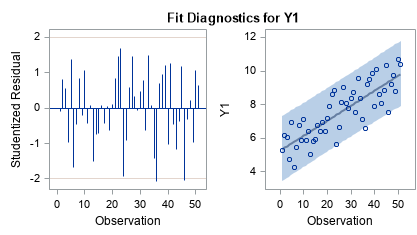
The AUTOREG procedure creates a panel of standard residual diagnostic plots. The panel includes a plot of the residuals and a fit plot that shows the fitted model and the observed values. For the linear data, the residual plots seem to indicate that the model fits the data well:

In contrast, the same residual panel for the quadratic data indicates a systematic pattern in the residuals:

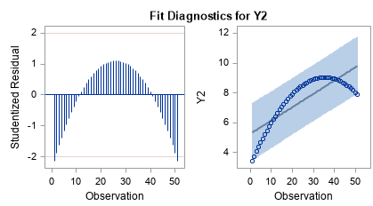
If this were a least squares model, which assumes independence of the residuals, those residual plots would indicate that this data-model combination does not satisfy the assumptions of the least squares regression model. For an autoregressive model, however, raw residuals can be correlated and exhibit a pattern. To determine whether the model is misspecified, PROC AUTOREG supports a special kind of residual analysis that uses recursive residuals.

The recursive residual for the k_th point is formed by fitting a line to the first k-1 points and then forming a standardized residual for the k_th point. The complete formulas are in the AUTOREG documentation. Galpin and Hawkins (1984) suggest plotting the cumulative sums of the recursive residuals as a diagnostic plot. Galpin and Hawkins credit Brown, Durbin, and Evans (1975) with proposing the CUSUM plot of the recursive residuals. The statistics output from the AUTOREG procedure are different than those in Galpin and Hawkin, but the idea and purpose behind the CUSUM charts are the same.

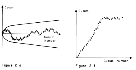
Galpin and Hawkin show a panel of nine plots that display different patterns that you might see in the CUSUM plots. I have reproduced two of the plots from the paper. (Remember, these graphs were produced in 1984!) The graph on the left shows what you should see for a correctly specified model. The cumulative sums stay within a region near the expected value of zero. In contrast, the graph on the right is one example of a CUSUM plot for a misspecified model.

The previous calls to PROC AUTOREG wrote the cumulative sums and the upper and lower boundaries of the confidence region to a data set. You can use PROC SGPLOT to create the CUSUM plot. The BAND statement is used to draw the confidence band:

ods layout gridded columns=2 advance=table;
 proc sgplot data=CusumLinear noautolegend;
    band x=x lower=lower upper=upper;
    series x=x y=cusum / break markers;
    refline 0  /axis=y noclip;
    xaxis grid; yaxis grid;
 run;
 proc sgplot data=CusumQuad noautolegend;
    band x=x lower=lower upper=upper;
    series x=x y=cusum / break markers;
    refline 0  /axis=y noclip;
    xaxis grid; yaxis grid;
 run;
ods layout end;

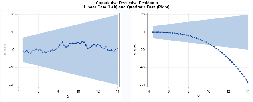
The graph on the left looks like a random walk on independent normal data. The cumulative sums stay within the colored confidence region. The model seems to fit the data. In contrast, the graph on the right quickly leaves the shaded region, which indicates that the model is misspecified.

In summary, there are many statistical tests that use a CUSUM statistic to determine whether deviations are random. These tests appear in many areas of statistics, including random walks, quality control, and time series analysis. For quality control, SAS supports the CUSUM procedure in SAS/QC software. For time series analysis, the AUTOREG procedure in SAS supports CUSUM charts of recursive residuals, which enable you to diagnose misspecified models.

You can download the SAS program that generates the graphs in this article.