I think every course in exploratory data analysis should begin by studying Anscombe's quartet. Anscombe's quartet is a set of four data sets (N=11) that have nearly identical descriptive statistics but different graphical properties. They are a great reminder of why you should graph your data. You can read about Anscombe's quartet on Wikipedia, or check out a quick visual summary by my colleague Robert Allison. Anscombe's first two examples are shown below:

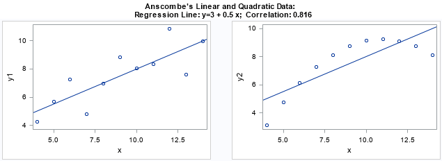
The Wikipedia article states, "It is not known how Anscombe created his data sets." Really? Creating different data sets that have the same statistics sounds like a fun challenge! As a tribute to Anscombe, I decided to generate my own versions of the two data sets shown in the previous scatter plots. The first data set is linear with normal errors. The second is quadratic (without errors) and has the exact same linear fit and correlation coefficient as the first data.

Generating your own version of Anscombe's data

The Wikipedia article notes that there are "several methods to generate similar data sets with identical statistics and dissimilar graphics," but I did not look at the modern papers. I wanted to try it on my own. If you want to solve the problem on your own, stop reading now!

I used the following approach to construct the first two data sets:

1. Use a simulation to create linear data with random normal errors: Y₁ = 3 + 0.5 X + ε, where ε ~ N(0,1).
2. Compute the regression estimates (b0 and b1) and the sample correlation for the linear data. These are the target statistics. They define three equations that the second data set must match.
3. The response variable for the second data set is of the form Y₂ = β₀ + β₁ X + β₂ X². There are three equations and three unknowns parameters, so we can solve a system of nonlinear equations to find β.

From geometric reasoning, there are three different solution for the β parameter: One with β₂ > 0 (a parabola that opens up), one with β₂ = 0 (a straight line), and one with β₂ < 0 (a parabola that opens down). Since Anscombe used a downward-pointing parabola, I will make the same choice.

Construct the first data set

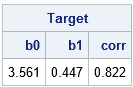
You can construct the first data set in a number of ways, but I choose to construct it randomly. The following SAS/IML statements construct the data, defines a helper function (LinearReg). The program computes the target values, which are the parameter estimates for a linear regression and the sample correlation for the data:

proc iml;
call randseed(12345);
x = T( do(4, 14, 0.2) );                              /* evenly spaced X */
eps = round( randfun(nrow(x), "Normal", 0, 1), 0.01); /* normal error */
y = 3 + 0.5*x + eps;                                  /* linear Y + error */
 
/* Helper function. Return paremater estimates for linear regression. Args are col vectors */
start LinearReg(Y, tX);
   X = j(nrow(tX), 1, 1) || tX;
   b = solve(X`*X, X`*Y);       /* solve normal equation */
   return b;
finish;
 
targetB = LinearReg(y, x);          /* compute regression estimates */
targetCorr = corr(y||x)[2];         /* compute sample correlation */
print (targetB`||targetCorr)[c={'b0' 'b1' 'corr'} F=5.3 L="Target"];

You can use these values as the target values. The next step is to find a parameter vector β such that Y₂ = β₀ + β₁ X + β₂ X² has the same regression line and corr(Y₂, X) has the same sample correlation. For uniqueness, set β₂ < 0.

Construct the second data set

You can formulate the problem as a system of equations and use the NLPHQN subroutine in SAS/IML to solve it. (SAS supports multiple ways to solve a system of equations.) The following SAS/IML statements define two functions. Given any value for the β parameter, the first function returns the regression estimates and sample correlation between Y₂ and X. The second function is the objective function for an optimization. It subtracts the target values from the estimates. The NLPHQN subroutine implements a hybrid quasi-Newton optimization routine that uses least squares techniques to find the β parameter that generates quadratic data that tries to match the target statistics.

/* Define system of simultaneous equations:
   https://blogs.sas.com/content/iml/2018/02/28/solve-system-nonlinear-equations-sas.html */
/* This function returns linear regression estimates (b0, b1) and correlation for a choice of beta */
start LinearFitCorr(beta) global(x);
   y2 = beta[1] + beta[2]*x + beta[3]*x##2;    /* construct quadratic Y */
   b = LinearReg(y2, x);      /* linear fit */
   corr = corr(y2||x)[2];     /* sample corr */
   return ( b` || corr);      /* return row vector */
finish;
 
/* This function returns the vector quantity (beta - target). 
   Find value that minimizes Sum | F_i(beta)-Target+i |^2 */
start Func(beta) global(targetB, targetCorr);
   target = rowvec(targetB) || targetCorr;
   G = LinearFitCorr(beta) - target;
   return( G );              /* return row vector */
finish;
 
/* now let's solve for quadratic parameters so that same 
   linear fit and correlation occur */
beta0 = {-5 1 -0.1};         /* initial guess */
con = {.  .  .,              /* constraint matrix */
       0  .  0};             /* quadratic term is negative */
optn = ncol(beta0) || 0;     /* LS with 3 components || amount of printing */
/* minimize sum( beta[i] - target[i])**2 */
call nlphqn(rc, beta, "Func", beta0, optn) blc=con;  /* LS solution */
print beta[L="Optimal beta"];
 
/* How nearly does the solution solve the problem? Did we match the target values? */
Y2Stats = LinearFitCorr(beta);
print Y2Stats[c={'b0' 'b1' 'corr'} F=5.3];

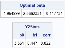
The first output shows that the linear fit and correlation statistics for the linear and quadratic data are identical (to 3 decimal places). Anscombe would be proud! The second output shows the parameters for the quadratic response: Y₂ = -4.955 + 2.566*X - 0.118*X². The following statements create scatter plots of the new Anscombe-like data:

y2 = beta[1] + beta[2]*x + beta[3]*x##2;
create Anscombe2 var {x y y2};  append;  close;
QUIT;
 
ods layout gridded columns=2 advance=table;
proc sgplot data=Anscombe2 noautolegend;
   scatter x=X y=y;    lineparm x=0 y=3.561 slope=0.447 / clip;
run;
proc sgplot data=Anscombe2 noautolegend;
   scatter x=x y=y2;   lineparm x=0 y=3.561 slope=0.447 / clip;
run;
ods layout end;

Notice that the construction of the second data set depends only on the statistics for the first data. If you modify the first data set, and the second will automatically adapt. For example, you could choose the errors manually instead of randomly, and the statistics for the second data set should still match.

What about the other data sets?

You can create the other data sets similarly. For example:

• For the data set that consist of points along a line except for one outlier, there are three free parameters. Most of the points fall along the line Y₃ = a + b*X and one point is at the height Y₃ = c. Therefore, you can run an optimization to solve for the values of (a, b, c) that match the target statistics.
• I'm not sure how to formulate the requirements for the fourth data set. It looks like all but one point have coordinates (X, Y₄), where X is a fixed value and the vertical mean of the cluster is c. The outlier has coordinate (a, b). I'm not sure whether the variance of the cluster is important.

Summary

In summary, you can solve a system of equations to construct data similar to Anscombe's quartet. By using this technique, you can create your own data sets that share descriptive statistics but look very different graphically.

To be fair, the technique I've presented does not enable you to reproduce Anscombe's quartet in its entirety. My data share a linear fit and sample correlation, whereas Anscombe's data share seven statistics!

Anscombe was a pioneer (along with Tukey) in using computation to assist in statistical computations. He was also enamored with the APL language. He introduced computers into the Yale statistics department in the mid-1960s. Since he published his quartet in 1973, it is possible that he used computers to assist his creation of the Anscombe quartet. However he did it, Anscombe's quartet is truly remarkable!

You can download the SAS program that creates the results in this article.