In my book Simulating Data with SAS, I show how to use a graphical tool, called the moment-ratio diagram, to characterize and compare continuous probability distributions based on their skewness and kurtosis (Wicklin, 2013, Chapter 16). The idea behind the moment-ratio diagram is that skewness and kurtosis are essential for understanding the shapes of many common univariate distributions. The skewness and kurtosis are sometimes called moment ratios because they are ratios of centralized moments of a distribution. A moment-ratio diagram displays the locus of possible (skewness, kurtosis) pairs for many common distributions. This article displays a simple moment-ratio diagram and shows the locations of a few well-known distributions.

Constructing the moment-ratio diagram

When you specify the parameters for a probability distribution, you get a density curve that has a particular shape. (The shape does not depend on the mean or variance, so all distributions in this article are assumed to be centered and scaled so that they have zero mean and unit variance.) The shape is partially characterized by the skewness and kurtosis values, although those two moments do not fully define the shape of the distribution.

For most probability distributions, the skewness and kurtosis depend on the distribution parameters. In general, the following is true:

• A distribution that has no shape parameters corresponds to a point in the moment-ratio (M-R) diagram.
• A distribution that has one shape parameter corresponds to a curve in the M-R diagram.
• A distribution that has two shape parameters corresponds to a region.

However, notice the phrase "shape parameters." A shape parameter changes the shape of the distribution, and not every parameter changes the shape. For example, location and scale parameters do not change the shape. The normal distribution has two parameters (location and scale), but all normal distributions are "bell-shaped." Because all normal curves have zero skewness and zero kurtosis, the normal distribution is represented by the point (0, 0) in the moment-ratio diagram. Similarly, the exponential distribution has a scale parameter, but all standardized exponential distributions have the same shape; the exponential distribution is represented by the point (2, 6) in the (skewness, kurtosis) coordinates.

In contrast, distributions such as the gamma or beta distributions have shape parameters that change the shape of the density function. The gamma distribution has one shape parameter and corresponds with a curve in the moment-ratio diagram. The beta distribution has two shape parameters and corresponds with a region in the moment-ratio diagram.

A basic moment-ratio diagram

This section lists a few common univariate distributions and specifies how the skewness and (excess) kurtosis depend on the parameters for the distributions. A simplified moment-ratio diagram appears to the right and displays points, curves, or regions for each distribution. Some researchers show only the right half of the diagram because many common distributions have positive skewness. By historical convention, the kurtosis axis points down. The letters and colors in the diagram are explained in the following list.

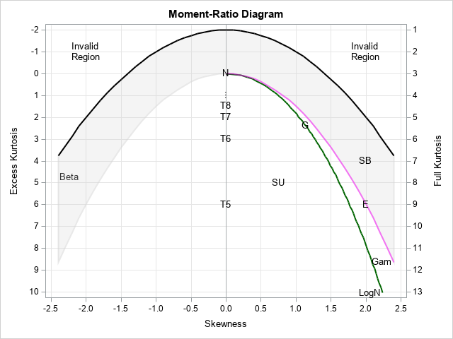
• Beta distribution: The beta distribution contains two parameters that affect the shape. The skewness and kurtosis range over a region (grey) that is bounded by two quadratic curves.
• Exponential distribution: Regardless of the value of the scale parameter, the skewness is always 2 and the kurtosis is always 6. Thus, the exponential distribution corresponds to a single point (E) on the M-R diagram.
• Gamma distribution: For the parameter α, the skewness is 2/sqrt(α) and the kurtosis is 6/α. Thus, the gamma distribution corresponds to a curve (magenta) on the M-R diagram. The centered gamma distribution converges to the normal distribution as α → ∞, which is why the gamma curve approaches the Normal point (N). The gamma distribution is also a limit of the beta distribution, which is why the gamma curve bounds the beta region.
• Gumbel distribution: The skewness is 1.14 and the kurtosis is 2.4. Thus, the Gumbel distribution corresponds to a single point (G).
• Lognormal distribution: The skewness is (exp(σ²) + 2) sqrt(exp(σ²) - 1). The kurtosis is exp(4σ²) + 2 exp(3σ²) + 3 exp(2σ²) - 6. Thus, the lognormal distribution corresponds to a curve (green) in the M-R diagram.
• Normal distribution: Every normal distribution has the same shape. The skewness and kurtosis are both 0 so there is a single point (N). The normal distribution is a limiting form of several distributions, including the beta, gamma, lognormal, and t.
• t distribution: The moments for the t distribution are only defined for more than four degrees of freedom (ν). For those distributions, the skewness is 0 and the kurtosis is 6/(ν - 4). Thus, the t distribution corresponds to a sequence of points (T5, T6, T7, ...) that converge to the normal distribution as ν → ∞.
• Johnson SB distribution: The Johnson SB distribution is a flexible distribution that can obtain any skewness and kurtosis combination "above" the lognormal distribution. Notice that this region overlaps with the beta region and the gamma curve. The overlap means that there are parameters for the SB distribution that have the same skewness and kurtosis as certain beta and gamma distributions. This does not imply that every distribution above the lognormal curve is a member of the SB family! It merely means that there is an SB distribution that has the same skewness and kurtosis.
• Johnson SU distribution: The Johnson SB distribution is a flexible distribution that can obtain any skewness and kurtosis combination "below" the lognormal distribution.

A more complex moment-ratio diagram

The moment-ratio diagram was known to early researchers such as Pearson in the 1800s. In 2010, E. Vargo, R. Pasupathy, and L. Leemis published a tour-de-force moment-ratio diagram that included dozens of probability distributions on one diagram ("Moment-Ratio Diagrams for Univariate Distributions", JQT, 2010). Read their paper to learn more about moment-ratio diagrams. Leemis provides a large color version of the moment-ratio diagram on his website and posted it in a 2019 article in Significance magazine. A low-resolution version is shown below. Click the image to see the original version.

What is the moment-ratio diagram used for?

The moment-ratio diagram is a useful theoretical tool for understanding the relationships between continuous univariate distributions. But how is the moment-ratio diagram useful to a data analyst? As I show in my book, you can use the moment-ratio diagram as a tool for modeling univariate distributions. Given a set of data, you can compute the sample skewness and kurtosis. By plotting the sample moments on the moment-ratio diagram, you can select candidate distributions to model the data. You can also use the moment-ratio diagram to organize simulation studies for which you want to test an algorithm or statistical method on data that have a wide range of skewness and kurtosis values.

An appendix to my book provides a SAS program that generates a moment-ratio diagram and overlays one or more data values. I used a small modification of that program to create the basic moment-ratio diagram in this article.