A SAS programmer wanted to simulate samples from a family of Beta(a,b) distributions for a simulation study. (Recall that a Beta random variable is bounded with values in the range [0,1].) She wanted to choose the parameters such that the skewness and kurtosis of the distributions varied over range of skewness-kurtosis pairs. How can you choose parameter values such that the skewness and kurtosis achieve a wide range of possible values?
The moment-ratio diagram is a statistical tool that helps to understand how to answer this question. This article shows how to use the moment-ratio diagram to find parameter values for the Beta(a,b) distribution that achieve a wide range of skewness-kurtosis values. The same ideas apply to finding parameters for other distributions. Recall that the full kurtosis is 3 more than the excess kurtosis. Both are popular measures, but in this article, "kurtosis" refers to the full kurtosis.
The moment-ratio diagram
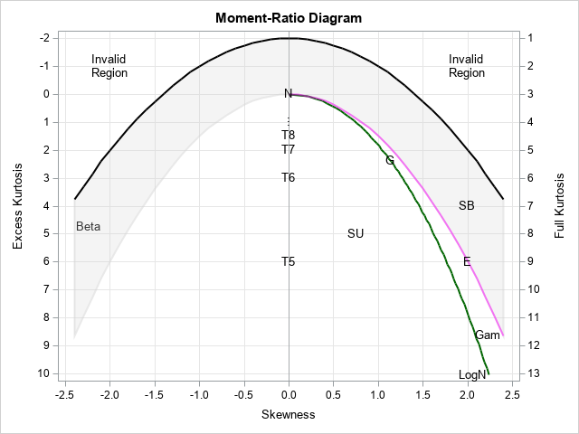
The moment-ratio diagram shows the range of possible skewness and kurtosis values ((s,k) values, for short) for many common families of probability distributions. Some families (such as the normal distribution) can only achieve a single (s,k) value. Other families (such as the gamma distribution) can achieve (s,k) values along a curve. Other families (such as the beta distribution) can achieve (s,k) values in a region.
In the diagram to the right, the gray region corresponds to the possible (s,k) values for the Beta distribution.
You can look up the formulas for the skewness and kurtosis of the Beta(a,b) distribution. The formulas for a > 0 and b > 0 are
Skewness: s(a,b) = ( 2 (b-a) sqrt(a+b+1) ) / ( (a+b+2) sqrt(a b) )
Full Kurtosis: k(a,b) = 3 + 6 ( (a-b)2 (a+b+1) - a b (a+b+2) ) /
( a b (a+b+2) (a+b+3) )
In other words, the gray region in the moment-ratio diagram is the image of the parameter region {(a,b) | a > 0, b > 0} under the nonlinear transformation (a,b) → (s,k).
Representative skewness-kurtosis values for the Beta distribution
The equations that define the Beta region in the moment-ratio diagram are well known.
The lower bound of the Beta region is the boundary of the "impossible region," so
k > 1 + s2
as it is for all distributions. The upper bound of the Beta region is the curve defined by the gamma distribution family, so
k < 3 + 1.5 s2.
Consequently, a good choice for a "representative" curve of (s,k) values for the beta distribution is the average of the two boundary curves, which is
k = 2 + 1.25 s2.
It suffices to consider only nonnegative skewness because if X is a Beta-distributed random variable that has skewness s, then 1-X is a beta-distributed variable that has skewness -s. Symmetric distributions (s=0) occur when a=b.
The following set of evenly spaced skewness values are a good choice for simulating random samples from the Beta distribution that have a wide range of skewness (s) and kurtosis (k) values:
/* specify values in the moment-ratio diagram for which the Beta distribution has a variety of (s,k) values */ data SKBetaParms; do s = 0 to 2.4 by 0.1; s = round(s,0.1); k = 2 + 1.25 * s**2; /* middle of the Beta region */ output; end; run; |
Solving for (a,b) values from (s,k) values
For each (s,k) value in the moment-ratio diagram, you can find the corresponding (a,b) parameter value for the Beta distribution that has the specified skewness and kurtosis. You can do this by solving for the root of the vector-valued function M(a,b) - (s,k), where M(a,b) is the transformation that maps parameter values to the corresponding (s,k) values. This can be done by using the SAS IML language, which enables you to define the vector-valued mapping and solve nonlinear equations in a least-square sense.
The steps in the process are as follows:
- Define a function (SKBetaFun) that takes an (a,b) input value and returns an (s,k) value as output.
- Define a function (VecFun) that evaluates the vector-valued function M(a,b) - (s,k).
- Define a function (SolveForBetaParam) that takes an (s,k) value and calls the NLPHQN subroutine in SAS IML to obtain an (a,b) value such that the norm of the VecFun function is minimized. Actually, SAS IML functions can take vectors of arguments, so the SolveForBetaParam can take vectors of several values and return several (a,b) values.
- For the (s,k) value in the SKBetaParms data set, call the SolveForBetaParam function to get the corresponding (a,b) parameters.
proc iml; /* Helper: return the skewness of the Beta(a,b) distribution */ start SkewBeta(a,b); return ( 2*(b-a)#sqrt(a+b+1) ) / ( (a+b+2)#sqrt(a#b) ); finish; /* Helper: return the full kurtosis of the Beta(a,b) distribution */ start KurtBeta(a,b); return 3 + 6* ( (a-b)##2 # (a+b+1) - a#b#(a+b+2) ) / ( a#b#(a+b+2)#(a+b+3) ); finish; /* 1. Define a function takes an (a,b) value and returns an (s,k) value */ start SKBetaFun(a,b); return ( SkewBeta(a,b) || KurtBeta(a,b) ); /* return a ROW vector */ finish; /* 2. Define a function that evaluates the vector-valued function M(a,b) - (s,k) */ start VecFun(param) global(g_skewTarget, g_kurtTarget); a = param[1]; b = param[2]; target = g_skewTarget || g_kurtTarget; return( SKBetaFun(a,b) - target ); finish; /* 3. Define a function that takes a vector of (s,k) values and calls the NLPHQN subroutine in SAS IML to obtain (a,b) values that minimize the norm of the VecFun function */ start SolveForBetaParam(skew, kurt, printLevel=0) global(g_skewTarget, g_kurtTarget); /* a b constraints. Lower bounds in 1st row; upper bounds in 2nd row */ con = {1e-6 1e-6, /* a > 0 and b > 0 */ . . }; x0 = {1 1}; /* initial guess */ optn = 2 // /* solve least square problem that has 2 components */ printLevel; /* amount of printing */ ab = j(nrow(skew), 2, .); /* return the a and b vectors as columns in matrix */ do i = 1 to nrow(skew); g_skewTarget = skew[i]; g_kurtTarget = kurt[i]; call nlphqn(rc, Soln, "VecFun", x0, optn) blc=con; /* solve for LS soln */ if rc>0 then ab[i,] = Soln; end; return( ab ); finish; |
You can read in the skewness-kurtosis pairs for the moments of the Beta distribution, then call the SolveForBetaParam function to obtain the corresponding (a,b) pairs:
/* 4. use values of (skew, kurt) that are in the middle of the Beta region. Solve for (a,b) parameters. */ use SKBetaParms; read all var {'s' 'k'}; close; Soln = SolveForBetaParam(s, k); a = Soln[,1]; b = Soln[,2]; print s k a[F=5.2] b[F=5.2]; |
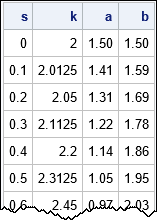
A few of the (a,b) parameter values are shown. For example, the parameter a = b = 1.5 define a symmetric Beta distribution that has full kurtosis equal to 2. The Beta(1.14, 1.86) distribution as skewness=0.4 and full kurtosis=2.2.
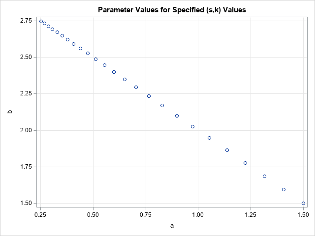
The (a,b) pairs are the preimage of points on the skewness-kurtosis curve in the center of the Beta region in the moment-ratio diagram. It isn't apparent from the table, but the preimage is a straight line in the (a,b) parameter space, as shown by the following graph. Notice, however, that the (a,b) values are not uniformly distributed along the line.
Visualizing the Beta distributions
Now that we know the (a,b) values that correspond to the specified values of skewness and kurtosis, what do these distributions look like? One way to visualize the distributions is to plot the PDF for a several (a,b) pairs. The following statements write the (a,b) pairs to a SAS data set, then creates a graph that overlays only four density curves for which the distribution has skewness values in the set {0, 0.5, 1, 2}. Each PDF is labeled by its parameters:
/* what do the curves look like? */ create Params var {'s' 'k' 'a' 'b'}; append; close; QUIT; data PDF; set Params(WHERE=(s in (0, 0.5, 1, 2))); /* display these four curves */ /* https://blogs.sas.com/content/iml/2018/08/08/plot-curves-two-categorical-variables-sas.html */ Group = catt("(a,b) = (", putn(a,5.2)) || "," || catt(putn(b,5.2)) || ")"; do x = 0.001, 0.005, 0.01 to 0.99 by 0.01, 0.999; PDF = pdf("Beta", x, a,b); output; end; run; title "Four Beta Distributions with Specified Skewness and Kurtosis"; title2 "Skewness = {0, 0.5, 1, 2}"; proc sgplot data=PDF; series x=x y=PDF / group=Group; xaxis grid; yaxis grid min=0 max=5; run; |
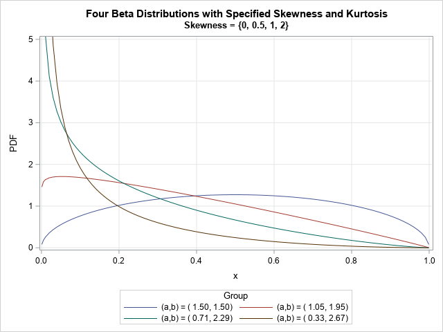
The graph shows one symmetric Beta PDF function and other function that have various amounts of positive skewness.
Summary
The moment-ratio diagram shows the possible skewness and kurtosis values for probability distributions. For example, the beta region is a U-shaped region. For each (s,k) pair in the moment-ratio diagram, there is a corresponding pair of parameter values, (a,b), such that Beta(a,b) has skewness=s and kurtosis=k. You can use nonlinear least squares optimization to find the (a,b) parameters for each feasible (s,k) value. This article uses SAS to find (a,b) parameter values for a range of (s,k) values. After you have obtained the (a,b) values, you can use them to simulate random Beta samples as part of a simulation study.

2 Comments
Pingback: Use the moment-ratio diagram to visualize the sampling distribution of skewness and kurtosis - The DO Loop
Pingback: Bimodal and unimodal beta distributions - The DO Loop