This article shows how to use SAS to solve a system of nonlinear equations. When there are n unknowns and n equations, this problem is equivalent to finding a multivariate root of a vector-valued function F(x) = 0 because you can always write the system as
f₁(x1, x2, ..., xn) = 0
f₂(x1, x2, ..., xn) = 0
. . .
f_n(x1, x2, ..., xn) = 0
Here the f_i are the nonlinear component functions, F is the vector (f₁, f₂, ..., f_n), and x is the vector (x1, x2, ..., xn).

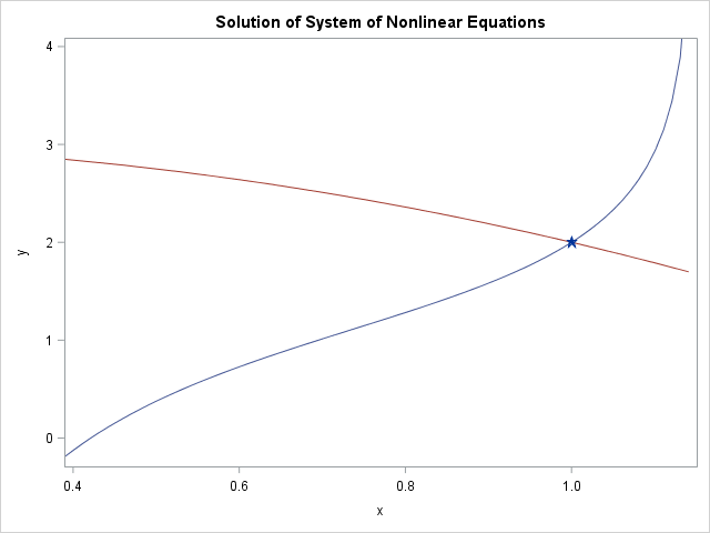
In two dimensions, the solution can be visualized as the intersection of two planar curves. An example for n = 2 is shown at the right. The two curves meet at the solution (x, y) = (1, 2).

There are several ways to solve a system of nonlinear equations in SAS, including:

• In SAS/IML software, you can use the NLPLM or NLPHQN methods to solve the corresponding least-squares problem. Namely, find the value of x that minimizes || F(x) ||.
• In SAS/ETS software, you can use the SOLVE statement in PROC MODEL to solve the system.
• In SAS/STAT software, you can use the NLIN procedure to solve the system.
• In SAS/OR software, you can use PROC OPTMODEL to solve the system.

When n = 1, the problem is one-dimensional. You can use the FROOT function in SAS/IML software to find the root of a one-dimensional function. You can also use the SOLVE function in conjunction with PROC FCMP.

This article shows how to find a root for the following system of three equations:
f₁(x, y, z) = log(x) + exp(-x*y) - exp(-2)
f₂(x, y, z) = exp(x) - sqrt(z)/x - exp(1) + 2
f₃(x, y, z) = x + y - y*z + 5
You can verify that the value (x, y, z)=(1, 2, 4) is an exact root of this system.

Solve a system of nonlinear equations in SAS/IML

You can use the NLPLM or NLPHQN methods in SAS/IML to solve nonlinear equations. You need to define a function that returns the value of the function as a vector. If the domain of any component of the function is restricted (for example, because of LOG or SQRT functions), you can define a linear constraint matrix. You then supply an initial guess and call the NLPLM routine to solve the least-squares problem that minimizes 1/2 (f₁² + ... + f_n²). Obviously the minimum occurs when each component is zero, that is, when (x,y,z) is a root of the vector-valued function. You can solve for the root as follows:

proc iml;
start Fun(var);
   x = var[1]; y = var[2]; z = var[3];
   f = j(1, 3, .);         /* return a ROW VECTOR */
   f[1] = log(x) + exp(-x*y) - exp(-2);
   f[2] = exp(x) - sqrt(z)/x - exp(1) + 2;
   f[3] = x + y - y*z  + 5;
return (f);
finish;
 
/*     x[1] x[2] x[3] constraints. Lower bounds in 1st row; upper bounds in 2nd row */
con = {1e-6  .  1e-6,   /* x[1] > 0 and x[3] > 0; no bounds on y */
         .   .    .};
x0 = {1 1 1};           /* initial guess */
optn = {3               /* solve least square problem that has 3 components */
        1};             /* amount of printing */
call nlphqn(rc, Soln, "Fun", x0, optn) blc=con;  /* or use NLPLM */
print Soln;
quit;

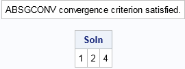
The NLPHQN routine converges to the solution (1, 2, 4). Notice that the first element of the optn vector must contain n, the number of equations in the system.

Solve a system of nonlinear equations with PROC MODEL

If you have access to SAS/ETS software, PROC MODEL provides a way to solve simultaneous equations. You first create a SAS data set that contains an initial guess for the solution. You then define the equations in PROC MODEL and use the SOLVE statement to solve the system, as follows:

data InitialGuess;
   x=1; y=1; z=1;    /* initial guess for Newton's method */
run;
 
proc model data=InitialGuess;
   bounds 0 < x z;
   eq.one = log(x) + exp(-x*y) - exp(-2);
   eq.two = exp(x) - sqrt(z)/x - exp(1) + 2;
   eq.three = x + y - y*z  + 5;
   solve x y z / solveprint out=solved outpredict;
run;quit;
 
title "Solution from PROC MODEL in SAS/ETS";
proc print data=solved noobs;
   var x y z;
run;

A nice feature of PROC MODEL is that it automatically generates symbolic derivatives and uses them in the solution of the simultaneous equations. If you want to use derivatives in PROC IML, you must specify them yourself. Otherwise, the NLP routines use numerical finite-difference approximations.

Solve a system of nonlinear equations with PROC NLIN

You can solve a system of equations by using only SAS/STAT software, but you need to know a trick. My colleague who supports PROC NLIN says he has "seen this trick before" but does not know who first thought of it. I saw it in a 2000 paper by Nam, Cho, and Shim (in Korean).

Because PROC NLIN is designed to solve regression problems, you need to recast the problem in terms of a response variable, explanatory variables, and parameters. Recall that ordinary least squares regression enables you to solve a linear system such as
0 = C1*v1 + C2*v2 + C3*v3
where the left-hand side is a response vector (the zero vector), the C_i are regression coefficients, and the v_i are explanatory variables. (You need three or more observations to solve this regression problem.) PROC NLIN enables you to solve more complex regression problems. In particular, the coefficients can be nonlinear functions of parameters. For example, if the parameters are (x,y,z), you can solve the following system:
0 = C1(x,y,z)*v1 + C2(x,y,z)*v2 + C3(x,y,z)*v3.

To solve this nonlinear system of equations, you can choose the explanatory variables to be coordinate basis functions: v1=(1,0,0), v2=(0,1,0), and v3=(0,0,1). These three observations define three equations for three unknown parameters. In general, if you have n equations in n unknowns, you can specify n coordinate basis functions.

To accommodate an arbitrary number of equations, the following data step generates n basis vectors, where n is given by the value of the macro variable numEqns. The BasisVectors data set contains a column of zeros (the LHS variable):

%let numEqns = 3;
data BasisVectors;
LHS = 0;
array v[&numEqns];
do i = 1 to dim(v);
   do j = 1 to dim(v);
      v[j] = (i=j);   /* 1 when i=j; 0 otherwise */
   end;
   output;
end;
drop i j;
run;
 
title "Solution from PROC NLIN in SAS/STAT";
proc nlin data=BasisVectors;
   parms x 1 y 1 z 1;                  /* initial guess */
   bounds 0 < x z;                     /* linear constraints */
   eq1 = log(x) + exp(-x*y) - exp(-2);
   eq2 = exp(x) - sqrt(z)/x - exp(1) + 2;
   eq3 = x + y - y*z  + 5;
   model LHS = eq1*v1 + eq2*v2 + eq3*v3;
   ods select EstSummary ParameterEstimates;
run;

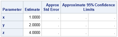
The problem contains three parameters and the data contains three observations. Consequently, the standard errors and confidence intervals are not meaningful. The parameter estimates are the solution to the nonlinear simultaneous equations.

Solve a system of nonlinear equations with PROC OPTMODEL

With PROC OPTMODEL in SAS/OR software, you can express the system in a natural syntax. You can either minimize the objective function F = 0.5 * (f1**2 + f2**2 + f3**2) or solve the system directly by specifying constraints but not an objective function, as follows:

title "Solution from PROC OPTMODEL in SAS/OR";
proc optmodel;
   var x init 1, y init 1, z init 1;
   /*  -or-  var x >= 1e-6 init 1, y init 1, z >= 0 init 1;  to specify bounds */
   con c1: log(x) + exp(-x*y) = exp(-2);
   con c2: exp(x) - sqrt(z)/x = exp(1) - 2;
   con c3: x + y - y*z = -5;
   solve noobjective;
   print x y z;
quit;

The solution is (x,y,z)=(1,2,4) and is not shown.

Summary

In summary, there are multiple ways to solve systems of nonlinear equations in SAS. My favorite ways are the NLPHQN function in SAS/IML and the SOLVE statement in PROC MODEL in SAS/ETS. However, you can also use PROC NLIN in SAS/STAT software or PROC OPTMODEL in SAS/OR. When you need to solve a system of simultaneous nonlinear equations in SAS, you can choose whichever method is most convenient for you.