In a recent article, I graphed the PDF of a few Beta distributions that had a variety of skewness and kurtosis values. I thought that I had chosen the parameter values to represent a wide variety of Beta shapes. However, I was surprised to see that the distributions were all unimodal.
It is well known that the Beta(a,b) distribution can be unimodal or bimodal. It is bimodal and U-shaped when 0 < a < 1 and 0 < b < 1. Otherwise, the Beta distribution is generically unimodal, with an important exception being a=b=1, which is the uniform distribution. A unimodal distribution can be L-shaped (mode at x=0), J-shaped (mode at x=1), or A-shaped (mode in the middle). The transition between unimodality and bimodality occurs when a=1 or b=1.
The moment-ratio diagram is a statistical tool that helps you to generate distributions that have a range of skewness and kurtosis values. The Beta distribution occupies a region of the moment-ratio diagram. When using the moment-ratio diagram to plan a simulation study, you might want to simulate some distributions that are unimodal and others that are bimodal. This article displays the curve in the moment-ratio diagram that separates the unimodal Beta distributions from the bimodal distributions. That curve is the image of the line segment {(a,1) | 0 < a < 1} under the mapping that maps the (a,b) parameter space into the (skewness, kurtosis) space.
The transformation into skewness-kurtosis space

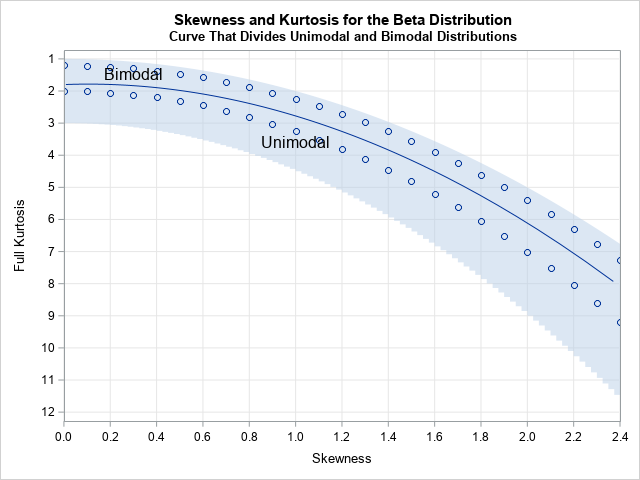
Let's jump to the result: The moment-ratio diagram to the right show the skewness-kurtosis region ((s,k) region, for short) for the Beta(a,b) distribution. The curve separates the region into two parts. The upper region is the set of (s,k) values for which the Beta distribution is U-shaped and bimodal. The lower region is the set of (s,k) values for which the Beta distribution is unimodal.
The Appendix has a link to the SAS code that creates this graph.
How are these regions computed? Well,
as mentioned in
a previous article,
the gray region in the moment-ratio diagram is the image of the parameter space {(a,b) | a > 0, b > 0}
under the transformation that maps (a,b) parameter values to (s,k) values, where s is the skewness of the Beta(a,b) distribution and k is the (full) kurtosis. Recall that
the formulas for the skewness and kurtosis of the Beta(a,b) distribution are
Skewness: s(a,b) = ( 2 (b-a) sqrt(a+b+1) ) / ( (a+b+2) sqrt(a b) )
Full Kurtosis: k(a,b) = 3 + 6 ( (a-b)2 (a+b+1) - a b (a+b+2) ) /
( a b (a+b+2) (a+b+3) )
If M is the name of the transformation that maps (a,b) to (s,k), then the curve in the middle of the gray region is the image M(A) of the open line segment A = {(a,b) | 0 < a < 1, b=1}. To get a bimodal distribution, chose a < 1 and b < 1. Equivalently, choose (s,k) values that are above the curve. To get a unimodal distribution, chose a > 1 or b > 1. Equivalently, choose (s,k) values that are below the curve.
As far as I can tell, the curve does not have a simple equation in (s,k) space. It is not a quadratic curve of k as a function of s.
How to ensure unimodal and bimodal Beta distributions?
You can use the curve in the moment-ratio diagram to ensure that you include both unimodal and bimodal distributions in a simulation study. For each value of skewness, you can choose a kurtosis value that is above the curve and another that is below the curve.
We already know that the quadratic curve in the "middle" of the Beta region is associated only with unimodal distributions. That is, for each skewness value (the horizontal coordinate), you can choose a value for the kurtosis (the vertical coordinate) that is 50% of vertical distance of the Beta region.
To get a bimodal distribution, you must choose a kurtosis that is closer to the "impossible region." If the skewness is not too large, there is a simple way to choose the kurtosis value. For each skewness value (the horizontal coordinate), you can choose a value for the kurtosis (the vertical coordinate) that is 10% of vertical distance of the Beta region for that skewness value. The result is shown in the graph below.
To be explicit,
for a given value of skewness, s, the point, (s,k), in the bimodal region satisfies the equation
k = (9/10) kLow + (1/10) kHigh
where
kLow = 1 + s2
is the boundary of the impossible region and
kHigh = 3 + 1.5 s2
is the opposite side of the Beta region. For comparison, the points in the unimodal region satisfy the equation k = (1/2) kLow + (1/2) kHigh.
Examples of unimodal and bimodal Beta distributions
Suppose you are interested in two Beta distributions—one unimodal and one bimodal—that have the same skewness, but one is unimodal and the other is bimodal. What do these distributions look like? To visualize the two Beta distributions, you can follow the method described in a previous article. Briefly, for each skewness-kurtosis value, (s,k), you must "pull back" the point into the parameter space for the Beta distribution. This results in a unique pair of (a,b) parameters. You can then plot the corresponding Beta(a,b) distribution. I won't repeat the computation, but here are the results for the following parameters:
- The point (s,k) = (1, 2.25) is in the bimodal region. The corresponding Beta parameters are (0.09, 0.24).
- The point (s,k) = (1, 3.25) is in the unimodal region. The corresponding Beta parameters are (0.71, 2.29).
The previous article also shows the SAS code to visualize these two Beta densities. The graph follows:
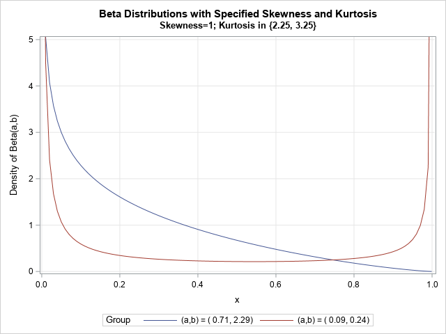
Note that the U-shaped graph is not symmetric. It might surprise you that these two distributions both have the same positive skewness, but they do. On the other hand, the kurtosis of the unimodal distribution is greater than the kurtosis of the bimodal distribution.
Summary
The Beta(a,b) distribution can assume several shapes. When (a,b) is in the unit square {(a,b) | a < 1 and b < 1}, the distribution is bimodal; otherwise, it is unimodal. The unit square corresponds to a strip in the moment-ratio diagram. Its complement is also mapped to a strip. If you want to include bimodal samples in a simulation study, you should be aware of these strips.
Although this article is specific to Beta distributions, the same ideas apply to other distributions. For examples, if you use the Johnson system to simulate data for a study, the Johnson SB distribution also has a unimodal and a bimodal region.
Appendix: The SAS code
You can download the SAS program that creates the graphs in this article from GitHub.
