From the early days of probability and statistics, researchers have tried to organize and categorize parametric probability distributions. For example, Pearson (1895, 1901, and 1916) developed a system of seven distributions, which was later called the Pearson system. The main idea behind a "system" of distributions is that for each feasible combination of skewness and kurtosis, there is a member of the system that achieves the combination. A smaller system is the Johnson system (Johnson, 1949), which contains only four distributions: the normal distribution, the lognormal distribution, the SB distribution (which models bounded distributions), and the SU distribution (which models unbounded distributions).

Every member of the Johnson system can be transformed into a normal distribution by using elementary functions. Because the transformation is invertible, it is also true that every member of the Johnson system is a transformation of a normal distribution.

The Johnson SB and SU distributions have four parameters and are extremely flexible, which means that they can fit a wide range of distribution shapes. As John von Neumann once said, "With four parameters, I can fit an elephant and with five I can make him wiggle his trunk." As I indicated in an article about the moment-ratio diagram, if you specify the skewness and kurtosis of a distribution, you can find a unique member of the Johnson system that has the same skewness and kurtosis.

This article shows how to compute the four essential functions for the Johnson SB distribution: the PDF, the CDF, the quantile function, and a method to generate random variates. It also shows how to fit the parameters of the distribution to data by using PROC UNIVARIATE in SAS.

What is the Johnson SB distribution?

The SB distribution contains a threshold parameter, θ, and a scale parameter, σ > 0. The SB distribution has positive density (support) on the interval (θ, θ + σ). The two shape parameters for the SB distribution are called δ and γ in the SAS documentation for PROC UNIVARIATE. By convention, the parameter δ is taken to be positive (δ > 0).

If X is a random variable from the Johnson SB distribution, then the variable
Z = γ + δ log( (X-θ) / (θ + σ - X) )
is standard normal. Because the transformation to normality is invertible, you can use properties of the normal distribution to understand properties of the SB distribution. The relationship also enables you to generate random variates of the SB distribution from random normal variates. To be explicit, define Y = (Z-γ) / δ, where Z ∼ N(0,1). Then the following transformation defines a Johnson SB random variable:
X = ( σ exp(Y) + θ (exp(Y) + 1) ) / (exp(Y) + 1);

Interestingly, if σ=1 and θ=0, then this is the logistic transformation. So one way to get a member of the Johnson system is as a logistic transformation of a normal random variable.

Generate random variates from the SB distribution

The relationship between the SB and the normal distribution provides an easy way to generate random variates from the SB distribution. You simply generate a normal variate and then transform it, as follows:

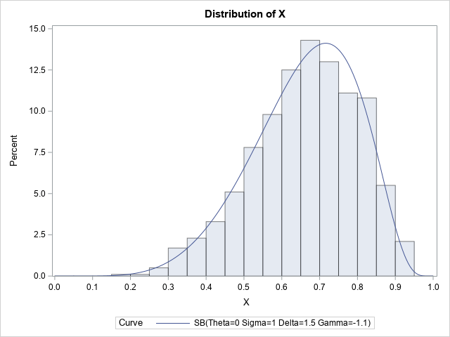
/* Johnson SB(threshold=theta, scale=sigma, shape=gamma, shape=delta) */
data SB(keep= X);
call streaminit(1);
theta = 0;   sigma = 1;   gamma = -1.1;    delta = 1.5;
do i = 1 to 1000;
   Y = (rand("Normal")-gamma) / delta;
   expY = exp(Y);
   X = ( sigma*expY + theta*(expY + 1) ) / (expY + 1);
   output;
end;
run;
 
/* set bins: https://blogs.sas.com/content/iml/2014/08/25/bins-for-histograms.html */
proc univariate data=SB;
   histogram X / SB(theta=0, sigma=1, gamma=-1.1, delta=1.5)
                 endpoints=(0 to 1 by 0.05);
   ods select Histogram;
run;

I used PROC UNIVARIATE in SAS to overlay the SB density on the histogram of the random variates. The result follows:

The PDF of the SB distribution

The formula for the SB density function is given in the PROC UNIVARIATE documentation (set h = v = 1 in the formula). You can evaluate the probability density function (PDF) on the interval (θ, θ + σ) in order to visualize the density function. So that you can easily compare various shape parameters, the following examples use θ=0 and σ=1 and plot the density on the interval (0, 1). The θ parameter translates the density curve and the σ parameter scales it, but these parameters do not change the shape of the curve. Therefore, only the two shape parameters are varied in the following program, which generates the PDF of the SB distribution for four combinations of parameters.

/* Visualize a few SB distributions */
data SB_pdf;
array _theta[4] _temporary_ (0 0 0 0);
array _sigma[4] _temporary_ (1 1 1 1);
array _gamma[4] _temporary_ (-1.1 -1.1  0.5  0.5);
array _delta[4] _temporary_ ( 1.5  0.8  0.8  0.05 );
sqrt2pi = sqrt(2*constant('pi'));
do i = 1 to dim(_theta);
   theta=_theta[i]; sigma=_sigma[i]; gamma=_gamma[i]; delta=_delta[i]; 
   Params = catt("gamma=", gamma, "; delta=", delta);
   do x = theta to theta+sigma by 0.005;
      c = delta / (sigma * sqrt2pi);
      w = (x-theta) / sigma;
      t = (x - theta) / (theta + sigma - x);
      PDF = c / (w*(1-w)) * exp( -0.5*(gamma + delta*log(t))**2 );
      output;
   end;
end;
drop c w t sqrt2pi;
run;
 
title "The Johnson SB Probability Density";
title2 "theta=0; sigma=1";
proc sgplot data=SB_pdf;
   label pdf="Density";
   series x=x y=pdf / group=Params lineattrs=(thickness=2);
   xaxis grid offsetmin=0 offsetmax=0;  yaxis grid;
run;

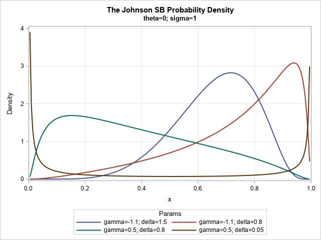
The graph shows that the SB distribution supports a variety of shapes. The blue curve (γ=–1.1, δ=1.5) and the red curve (γ=–1.1, δ=0.8) both exhibit negative skewness, whereas the green curve (γ=0.5, δ=0.8) has positive skewness. Those three curves are unimodal, whereas the brown curve (γ=0.5, δ=0.05) is a U-shaped distribution. These curves might remind you of the beta distribution, which is a more familiar family of bounded distributions.

The CDF and quantiles of the SB distribution

I am not aware of explicit formulas for the cumulative distribution function (CDF) and quantile function of the SB distribution. You can use numerical integration of the PDF to evaluate the cumulative distribution. You can use numerical root-finding methods to evaluate the inverse CDF (quantile) function, but it will be an expensive computation.

Fitting parameters of the SB distribution

If you have data, you can use PROC UNIVARIATE to estimate four parameters of the SB distribution that fit the data. In practice, often the threshold (and sometimes the scale) is known from domain-specific knowledge. For example, if you are modeling student test scores, you might know that the scores are always in the range [0, 100], so θ=0 and σ=100.

In an earlier section, we simulated a data set for which all values are in the interval [0, 1]. The following call to PROC UNIVARIATE estimates the shape parameters for these simulated data:

proc univariate data=SB;
   histogram X / SB(theta=0, sigma=1, fitmethod=moments) 
                 endpoints=(0 to 1 by 0.05);
run;

By default, the HISTOGRAM statement uses the FITMETHOD=PERCENTILE method to fit the data. You can also use FITMETHOD=MLE to obtain a maximum likelihood estimate, or FITMETHOD=MOMENTS to estimate the parameters by matching the sample moments. In this example, I show how to use the FITMETHOD=MOMENTS option, which, for these data, seems to provide a better fit than the method of percentiles.

Summary

The Johnson system is a four-parameter system that contains four families of distributions. If you choose any feasible combination of skewness and kurtosis, you can find a member of the Johnson system that has that same skewness and kurtosis. The SB distribution is a family that models bounded distributions. This article shows how to simulate random values from the SB distribution and how to visualize the probability density function (PDF). It also shows how to use PROC UNIVARIATE to fit parameters of the SB distribution to data.