When you run an optimization, it is often not clear how to provide the optimization algorithm with an initial guess for the parameters. A good guess converges quickly to the optimal solution whereas a bad guess might diverge or require many iterations to converge. Many people use a default value (such as 1) for all initial guesses. I have previously written about other ways to obtain an initial guess for an optimization.

In the special case of maximum likelihood estimation, you use a trick to provide a good guess to the optimization algorithm. For maximum likelihood estimation, the objective function is the log-likelihood function of a distribution. Consequently, you can use the method of moments to provide the initial guess for the parameters, which often results in fast convergence to the maximum likelihood estimates. The faster convergence can save you considerable time when you are analyzing thousands of data sets, such as during a simulation study.

The method of moments

Suppose you believe that some data can be modeled by a certain distribution such as a lognormal, Weibull, or beta distribution. A common way to estimate the distribution parameters is to compute the maximum likelihood estimates (MLEs). These are the values of the parameters that are "most likely" to have generated the observed data. To compute the MLEs you first construct the log-likelihood function and then use numerical optimization to find the parameter values that maximize the log-likelihood function.

The method of moments is an alternative way to fit a model to data. For a k-parameter distribution, you write the equations that give the first k central moments (mean, variance, skewness, ...) of the distribution in terms of the parameters. You then replace the distribution's moments with the sample mean, variance, and so forth. You invert the equations to solve for the parameters in terms of the observed moments.

For example, suppose you believe that some data are distributed according to a two-parameter beta distribution. If you look up the beta distribution on Wikipedia, you will see that the mean and variance of a Beta(a, b) distribution can be expressed in terms of the two parameters as follows:

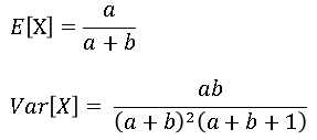
The first equation represents the expected (mean) value of a beta-distributed random variable X. The second equation represents the variance. If the sample mean of the data is m and the sample variance is v, you can "plug in" these values for the left-hand side of the equations and solve for the values of a and b that satisfy the equations. Solving the first equation for a yields a = b m / (1 - m). If you substitute that expression into the second equation and solve for b, you get b = m - 1 + (m/v)(1 - m)². Those equations give the parameter estimates from the method of moments.

Maximum likelihood estimation: Using an arbitrary guess

The method of moments can lead to improved convergence when fitting a distribution. For comparison, first consider what happens if you use an arbitrary initial guess for the optimization, such as a = b = 1. The following statements use PROC NLMIXED to compute maximum likelihood estimates for the parameters of the beta distribution. (You can read about how to use PROC NLMIXED to construct MLEs. You can also compute MLEs by using SAS/IML.)

data Beta;
input x @@;
datalines;
0.58 0.23 0.41 0.69 0.64 0.12 0.07 0.19 
0.47 0.05 0.76 0.18 0.28 0.06 0.34 0.52 
0.42 0.48 0.11 0.39 0.24 0.25 0.22 0.05 
0.23 0.49 0.45 0.29 0.18 0.33 0.09 0.16 
0.45 0.27 0.31 0.41 0.30 0.19 0.27 0.57 
;
 
/* Compute parameter estimates for the beta distribution */
proc nlmixed data=Beta;
   parms a=1 b=1;                /* use arbitrary initial guesses */
   bounds a b > 0;
   LL = logpdf("beta", x, a, b); /* log-likelihood function */
   model x ~ general(LL);
run;

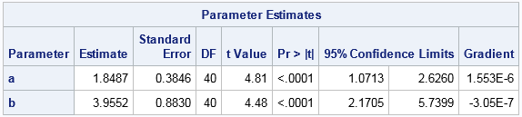
The MLEs are a = 1.8487 and b = 3.9552. The "Iteration History" table (not shown) shows that 8 iterations of a quasi-Newton algorithm were required to converge to the MLEs, and the objective function (the LOGPDF function) was called 27 times during the optimization.

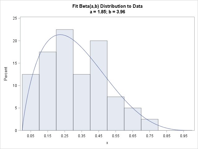
The following graph shows a histogram of the data overlaid with a Beta(a=1.85, b=3.96) density curve. The curve fits the data well.

Maximum likelihood estimation: Using method-of-moments for guesses

If you use the method-of-moments to provide an initial guess on the PARMS statement, the quasi-Newton algorithm might converge in fewer iterations. The following statements use PROC MEANS to compute the sample mean and variance, the use the DATA step to compute the method-of-moments estimates, as follows:

/* output mean and variance */
proc means data=Beta noprint;
   var x;
   output out=Moments mean=m var=v;  /* save sample moments */
run;
 
/* use method of moments to estimate parameters for the beta distribution */
data ParamEst;
   retain a b;               /* set order of output variables */
   set Moments;
   b = m*(1-m)**2/v + m - 1; /* estimate parameters by using sample moments */
   a = b*m / (1-m);
   keep a b;
run;

The method of moments estimates are a = 1.75 and b = 3.75, which are close to the MLE values. The DATA= option in the PARMS statement in PROC NLMIXED enables you to specify a data set that contains starting values for the parameters. The following call to PROC NLMIXED is exactly the same as the previous call except that the procedure uses the initial parameter values from the ParamEst data set:

proc nlmixed data=Beta;
   parms / data=ParamEst;        /* use initial guesses from method of moments */
   bounds a b > 0;
   LL = logpdf("beta", x, a, b); /* log-likelihood function */
   model x ~ general(LL);
run;

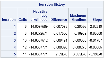
The MLEs from this call (not shown) are exactly the same as before. However, the "Iteration History" table indicates that quasi-Newton algorithm converged in 5 iterations and required only 14 calls the objective function. This compares with 8 iterations and 27 calls for the previous computation. Thus the method of moments resulted in about half as many functional evaluations. In my experience this example is typical: Choosing initial parameters by using the method of moments often reduces the computational time that is required to obtain the MLEs.

It is worth mentioning that the PARMS option in PROC NLMIXED supports two nice features:

• The DATA= option accepts both wide and long data sets. The example here is wide: there are k variables that supply the values of the k parameters. You can also specify a two-variable data set with the names "Parameter" and "Estimate."
• The BYDATA option enables you to specify initial guesses for each BY group. In simulation studies, you might use BY-group processing to compute the MLEs for thousands of samples. The BYDATA option is essential to improving the efficiency of a large simulation study. It can also help ensure that the optimization algorithm converges when the parameters for the samples range over a large set of values.

Summary and cautions

In summary, this article shows how to use the method of moments to provide a guess for optimizing a log-likelihood function, which often speeds up the time required to obtain the MLEs. The method requires that you can write the equations that relate the central moments of a distribution (mean, variance, ...) to the parameters for the distribution. (For a distribution that has k parameters, use the equations for the first k moments.) You then "plug in" the sample moments and algebraically invert the equations to obtain the parameter values in terms of the sample moments. This is not always possible analytically; you might need to use numerical methods for part of the computation.

A word of caution. For small samples, the method of moments might produce estimates that do not make sense. For example, the method might produce a negative estimate for a parameter that must be positive. In these cases, the method might be useless, although you could attempt to project the invalid parameters into the feasible region.