The moment-ratio diagram is a tool that is useful when choosing a distribution that models a sample of univariate data. As I show in my book (Simulating Data with SAS, Wicklin, 2013), you first plot the skewness and kurtosis of the sample on the moment-ratio diagram to see what common distributions have similar moments. These are candidate choices. However, you never should select a choice based only on the point estimates because the skewness and kurtosis statistics have large standard errors. That is why I recommend bootstrapping the data and plotting the bootstrap distribution of the skewness and kurtosis statistics. The cloud of points gives a much better indication of the possible distributions that might be appropriate models for the data.

Of course, the bootstrap distribution of the statistics is only an approximation to the true sampling distribution of the statistics, which you can visualize by using a simulation study. This article simulates random samples from a beta distribution and plots the sampling distribution of the skewness and kurtosis statistics on the moment-ratio diagram. This demonstrates the variability of the skewness and kurtosis statistics.

Simulate from a Beta distribution

A previous article describes the region of the moment-ratio diagram that corresponds to the Beta distribution. Let's use the parameter values a=0.705 and b=2.295. As shown in the previous article, the Beta(0.705, 2.295) distribution has skewness=1 and (full) kurtosis=3.25. Let's simulate 1,000 random samples from the Beta(0.705, 2.295) distribution and compute the skewness and kurtosis for each sample:

/* simulate NumSamples random samples of size N 
   from the Beta(a,b) distribution for each (a,b) value */
data Params;
   a=0.705; b=2.295;       /* define Beta parameters */
   s=1.0;   k=3.25;        /* moments of the Beta(a,b) distribution */
run;
 
%let NumSamples = 1000; /* number of Monte-Calo samples */
%let N = 50;            /* sample size */
data SimBeta;
set Params;
call streaminit(123);
do SampleID = 1 to &NumSamples;
   do i = 1 to &N;
      x = rand("Beta", a, b);
      output;
   end;
end;
keep SampleId i x;
run;
 
/* compute sample skewness and kurtosis for each sample */
proc means data=SimBeta noprint;
   by SampleID;
   var x;
   output out=SimDist skew=SampleSkew kurt=SampleExKurt;
run;
 
/* transform excess kurtosis to full kurtosis */
data SimDist;
set SimDist(drop=_TYPE_ _FREQ_);
SampleKurt = 3 + SampleExKurt;
run;

You can plot the sample statistics on the moment-ratio diagram to visualize their spread. Since we know these data are Beta-distributed, I will overlay only the Beta region of the moment-ratio diagram:

/* visualize the sample distributions on the moment-ratio diagram */
data BetaRegion;
do sx = 0 to 2.4 by 0.025;
   kLower = 1 + sx**2;     output;  /* boundary of impossible region */
   kUpper = 3 + 1.5*sx**2; output;  /* gamma line = boundry of Beta region */
end;
run;
 
data PlotData;
set Params SimDist BetaRegion;
run;
 
title "Distribution of Sample Skewness and Kurtosis";
title2 "&NumSamples Samples of Size N=*N, X ~ Beta(0.705, 2.295)";  
proc sgplot data=PlotData;
   band x=sx lower=kLower upper=kUpper / legendlabel="Beta Region" transparency=0.5;
   scatter x=SampleSkew y=SampleKurt / legendlabel="Sample Momemts";
   scatter x=s y=k / markerattrs=(symbol=StarFilled color=red) legendlabel="Moments of Distribution";
   yaxis grid reverse label="Full Kurtosis";
   xaxis grid label="Skewness";
run;

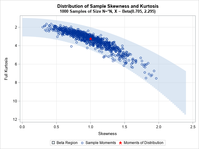
The graph shows the sample (skewness, kurtosis) statistics for 1,000 random samples of size N=50 from the Beta(0.705, 2.295) distribution. The skewness and kurtosis for the distribution itself is shown as a red star at (1, 3.25). The statistics for the samples vary greatly. Some are not even inside the Beta region! About 95% of the samples have a skewness in the interval [0.5, 1.6]. About 95% of the kurtosis values are in the interval [2, 5.7]. These are wide intervals, which shows the variability of these statistics for N=50. Of course, statistics for larger samples would have smaller variability.

Applications to modeling univariate data

The lesson to take away from this simulation experiment is that the skewness and kurtosis statistics have large standard errors. When you have a sample of real data (especially a small sample), you should not immediately choose the region or curve that is nearest to the sample statistics. Rather, you should bootstrap the data set to get a feel for the variation of the skewness and kurtosis statistics. You will often see a cloud of point similar to what is shown in this article. The cloud indicates plausible distributions that might model the data well.

Because there are so many distributions, it can be difficult to decide which is most appropriate for your data. In the absence of domain-specific knowledge about the data-generating process, some practitioners prefer to use a flexible distribution to model the data. A popular choice for a flexible distribution is the Johnson system, which covers the moment-ratio diagram by using only four distribution families: a bounded family (the Johnson SB distribution), an unbounded family (the Johnson SU distribution), the normal distribution, and the lognormal distribution. For multimodal distributions, some practitioners use the newer metalog system (Keelin, 2016).

Summary

This article uses simulation to visualize the spread of the skewness and kurtosis statistics for a Beta distribution. The distribution has skewness equal to 1 and (full) kurtosis equal to 3.25. Random samples of size N=50 have wide range of skewness and kurtosis statistics. Although most of the sample statistics are inside the Beta region of the moment-ratio diagram, not all are. Using the point estimates from one of these samples to choose the distribution to model the data is unwise. The careful analyst will instead bootstrap the data to get a better feel for the possible distributions that could reasonably model the data. The bootstrap distribution will look similar to the point cloud in this article.