The Johnson system: Which distribution should you choose to model data?

The Johnson system (Johnson, 1949) contains a family of four distributions: the normal distribution, the lognormal distribution, the SB distribution, and the SU distribution. Previous articles explain why the Johnson system is useful and show how to use PROC UNIVARIATE in SAS to estimate parameters for the Johnson SB distribution or for the Johnson SU distribution.

How to choose between the SU and SB distribution?

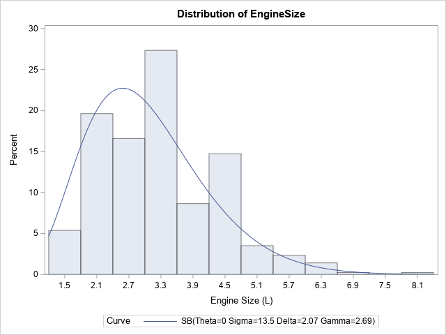
The graph to the right shows a histogram with an overlay of a fitted Johnson SB density curve. But why fit the SB distribution? Why not the SU? For a given sample of data, it is not usually clear from the histogram whether the tails of the data are best described as thin-tailed or heavy-tailed. Accordingly, it is not clear whether the SB (bounded) or the SU (unbounded) distribution is a more appropriate model.

One way to answer that question is to plot the sample kurtosis and skewness on a moment-ratio diagram to see if it is in the SB or SU region of the diagram. Unfortunately, high-order sample moments have a lot of variability, so this method is not very accurate. See Chapter 16 of Simulating Data with SAS for examples.

Slifker and Shapiro (1980) devised a method that does not use high-order moments. Instead, they compare the length of the tails of the distribution to the length of the central portion of the distribution. They use four quantiles to define "the tails" and "the central portion," so their method is similar to a robust definition of skewness, which also uses quantile information.

For ease of exposition, in this section I will oversimplify Slifker and Shapiro's results. Essentially, they suggest using the 6th, 30th, 70th, and 94th percentiles of the data to determine whether the data are best modeled by the SU, SB, or lognormal distribution. Denote these percentiles by P6, P30, P70, and P94, respectively. The key quantities in the computation are lengths of the intervals between percentiles of the data. In particular, define

m = P94 - P70 (the length of the upper tail)
n = P30 - P06 (the length of the lower tail)
p = P70 - P30 (the length of the central portion)

Slifker and Shapriro show that if you use percentiles of the distributions, the ratio m*n/p² has the following properties:

m*n/p² > 1 for percentiles of the SU distribution
m*n/p² < 1 for percentiles of the SB distribution
m*n/p² = 1 for percentiles of the lognormal distribution

Therefore, they suggest that you use the sample estimates of the percentiles to compute the ratio. If the ratio is close to 1, use the lognormal distribution. Otherwise, if the ratio is greater than 1, use the SU distribution. Otherwise, if the ratio is less than 1, use the SB distribution.

Details of the computation

The previous section oversimplifies one aspect of the computation. Slifker and Shapiro don't actually recommend using the 6th, 30th, 70th, and 94th percentiles of the data. They recommend choosing a normal variate, z (0 < z < 1) that depends on the size of the sample. They recommend using "a value of z near 0.5 such as z = 0.524" for "moderate-sized data sets" (p. 240). After choosing z, consider the evenly spaced values {-3*z, -z, z, 3*z}. These points divide the area under the normal density curve into four regions.

For z = 0.524, the areas of these regions are 0.058, 0.300, 0.700, and 0.942. These, then, are the quantiles to use for "moderate-sized data sets." This choice assumes that the 5.8th and 94.2th sample percentiles (which define the "tails") are good approximates of the percentiles of the distribution. If you have a large data set, another reasonable choice would be z = 0.6745, which leads to the 2.2th, 25th, 75th, and 97.8th percentiles.

A SAS program to determine the Johnson family from data

You can write a SAS/IML program that reads in univariate data, computes the percentiles of the data, and computes the ratio m*n/p². You can use the QNTL function in the SAS/IML language to compute the percentiles, but Slifker and Shapiro use a slightly nonstandard definition of percentiles in their paper. For consistency, the following program uses their definition. Part of the percentile computation requires looking at the integer and fractional part of a number.

The following program analyzes the EngineSize variable in the Sashelp.Cars data set:

/* For Sashelp.Cars, the EngineSize (and Cylinders) variable is SB. Others are SU. */
%let dsname = Sashelp.Cars;
%let varName = EngineSize; /* OR  %let varName = mpg_city; */
 
/* Implement the Slifker and Shapiro (1980) https://www.jstor.org/stable/1268463
   method that uses sample percentiles to assess whether the data are best 
   modeled by the SB, SU, or SL (lognormal) distributions. */
proc iml;
/* exclude any row with missing value: https://blogs.sas.com/content/iml/2015/02/23/complete-cases.html */
start ExtractCompleteCases(X);
   idx = loc(countmiss(X, "row")=0);
   if ncol(idx)>0 then return( X[idx, ] ); else return( {} ); 
finish;
 
/* read the variable into x */
use &dsname;
   read all var {&varName} into x;
close;
 
x = ExtractCompleteCases(x);      /* remove missing values */
if nrow(x)=0 then abort;
call sort(x);
N = nrow(x);
 
/* Generate the percentiles as percentiles of the normal distribution for evenly spaced 
   variates. This computation does not depend on the data values. */
z0 = 0.524;                       /* one possible choice. Another might be 0.6745 */
z = -3*z0 // -z0 // z0 // 3*z0;   /* evenly space z values */
pctl = cdf("Normal", z);          /* percentiles of the normal distribution */
print pctl[f=5.3];                /* These are the percentiles to use */
 
/* Note: for z0 = 0.524, the percentiles are approximately 
   the 5.8th, 30th, 70th, and 94.2th percentiles of the data */
 
/* The following computations are almost (but not quite) the same as 
   call qntl(xz, x, p);   
   Use MOD(k,1) to compute the fractional part of a number.  ‎*/
k = pctl*N + 0.5;
intk = int(k);          /* int(k) is integer part and mod(k,1) is fractional part */
xz = x[intk] + mod(k,1) # (x[intk+1] - x[intk]); /* quantiles using linear interpol */
 
/* Use xz to compare length of left/right tails with length of central region */
m = xz[4] - xz[3];      /* right tail: length of 94th - 70th percentile */
n = xz[2] - xz[1];      /* left tail: length of 30th - 6th percentile */
p = xz[3] - xz[2];      /* central region: length of 70th - 30th percentile */
 
/* use ratio to decide between SB, SL (lognormal) and SU distributions */
ratio = m*n/p**2;
eps = 0.05;             /* if ratio is within 1 +/- eps, use lognormal */
 
if (ratio > 1 + eps) then 
   type = 'SU';
else if (ratio < 1 - eps) then
   type = 'SB';
else 
   type = 'LOGNORMAL';
 
print type;
call symput('type', type);   /* optional: store value in a macro variable */
quit;

The output of the program is the word 'SB', 'SU', or 'LOGNORMAL', which indicates which Johnson distribution seems to fit the data. When you know this information, you can use the appropriate option in the HISTOGRAM statement of PROC UNIVARIATE. For example, the SB distribution seems to be appropriate for the EngineSize variable, so you can use the following statements to produce the graph at the top of this article.

proc univariate data=Sashelp.Cars;
   var EngineSize;
   histogram EngineSize / SB(theta=0 sigma=EST fitmethod=moments);
   ods select Histogram;
run;

Most of the other variables in the Sashelp.Cars data are best modeled by using the SU distribution. For example, if you change the value of the &varName macro to mpg_city and rerun the program, the program will print 'SU'.

Concluding thoughts

Slifker and Shapiro's method is not perfect. One issue is that you have to choose a particular set of percentiles (derived from the choice of "z0" in the program). Different choices of z0 could conceivably lead to different results. And, of course, the sample percentiles—like all statistics—have sampling variability. Nevertheless, the method seems to work adequately in practice.

The second part of Slifker and Shapiro describe a method of using the percentiles of the data to fit the parameters of the data. This is the "method of percentiles" that is mentioned in the PROC UNIVARIATE documentation. In a companion article, Mage (1980, p. 251) states: "Although a given percentile point fit of the SB parameters may be adequate for most purposes, the ambiguity of obtaining different parameters by different percentile choices may be unacceptable in some applications." In other words, it would be preferable to "avoid the situation where one choice of percentiles leads to [one conclusion]and a second choice of percentiles leads to [a different conclusion]."

It is worth noting that the UNIVARIATE procedure supports three different methods for fitting parameters in the Johnson distributions. No one method works perfectly for all possible data sets, so experiment with several different methods when you use the Johnson distribution to model data.

Blogs