The Johnson system (Johnson, 1949) contains a family of four distributions: the normal distribution, the lognormal distribution, the SB distribution (which models bounded distributions), and the SU distribution (which models unbounded distributions). Note that 'B' stands for 'bounded' and 'U' stands for 'unbounded.' A previous article explains the purpose of the Johnson system and shows how to work with the Johnson SB distribution, including how to compute the probability density function (PDF), generate random variates, and estimate parameters from data. This article provides similar information for the Johnson SU distribution.

What is the Johnson SU distribution?

The SU distribution contains a location parameter, θ, and a scale parameter, σ > 0. The SU density is positive for all real numbers. The two shape parameters for the SU distribution are called δ and γ in the SAS documentation for PROC UNIVARIATE. By convention, the δ parameter is taken to be positive (δ > 0).

If X is a random variable from the Johnson SU distribution, then the variable
Z = γ + δ sinh^-1( (X-θ) / σ )
is standard normal. The transformation to normality is invertible. Because sinh^-1(t) = arsinh(t) = log(t + sqrt(1+t²)), some authors specify the transformation in terms of logs and square roots.

Generate random variates from the SU distribution

The relationship between the SU and the normal distribution provides an easy way to generate random variates from the SU distribution. To be explicit, define Y = (Z-γ) / δ, where Z ∼ N(0,1). Then the following transformation defines a Johnson SU random variable:
X = θ + σ sinh(Y),
where sinh(t) = (exp(t) – exp(-t)) / 2.

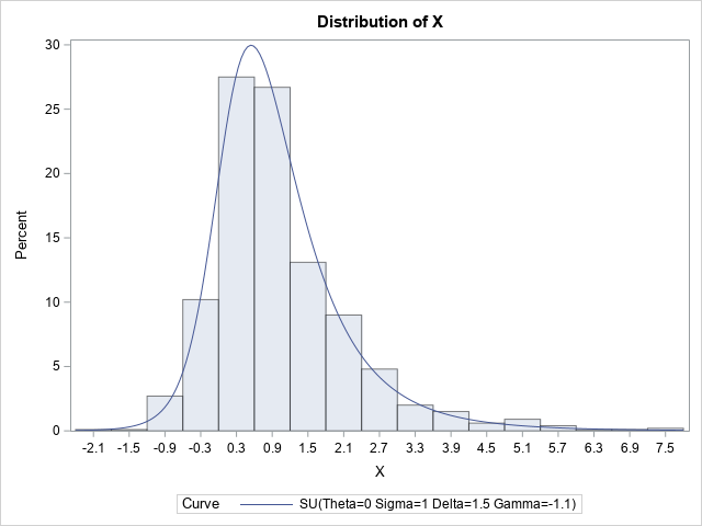
The following SAS DATA step generates a random sample from a Johnson SU distribution:

/* Johnson SU(location=theta, scale=sigma, shape=delta, shape=gamma) */
data SU(keep= X);
call streaminit(1);
theta = 0;  sigma = 1;   gamma = -1.1;   delta = 1.5;  
do i = 1 to 1000;
   Y = (rand("Normal")-gamma) / delta;
   X = theta + sigma * sinh(Y);
   output;
end;
run;

You can use PROC UNIVARIATE in SAS to overlay the SU density on the histogram of the random variates:

proc univariate data=SU;
   histogram x / SU(theta=0 sigma=1 gamma=-1.1 delta=1.5);
   ods select Histogram;
run;

The PDF of the SU distribution

The formula for the SU density function is given in the PROC UNIVARIATE documentation (set h = v = 1 in the formula). You can evaluate the probability density function (PDF) on the interval [θ – 4 σ, θ + 4 σ] for visualization purposes. So that you can easily compare various shape parameters, the following examples use θ=0 and σ=1. The θ parameter translates the density curve and the σ parameter scales it, but these parameters do not change the shape of the curve. Therefore, only the two shape parameters are varied in the following program, which generates the PDF of the SU distribution for four combinations of parameters.

/* Visualize a few SU distributions */
data SU_pdf;
array _theta[4] _temporary_ (0 0 0 0);
array _sigma[4] _temporary_ (1 1 1 1);
array _gamma[4] _temporary_ (-1.1 -1.1  0.5  0.5);
array _delta[4] _temporary_ ( 1.5  0.8  0.8  0.5 );
sqrt2pi = sqrt(2*constant('pi'));
do i = 1 to dim(_theta);
   theta=_theta[i]; sigma=_sigma[i]; gamma=_gamma[i]; delta=_delta[i]; 
   Params = catt("gamma=", gamma, "; delta=", delta);
   do x = theta-4*sigma to theta+4*sigma by 0.01;
      c = delta / (sigma * sqrt2pi);
      w = (x-theta) / sigma;
      z = gamma + delta*arsinh(w);
      PDF = c / sqrt(1+w**2) * exp( -0.5*z**2 );
      output;
   end;
end;
drop c w z sqrt2pi;
run;
 
title "The Johnson SU Probability Density";
title2 "theta=0; sigma=1";
proc sgplot data=SU_pdf;
   label pdf="Density";
   series x=x y=pdf / group=Params lineattrs=(thickness=2);
   xaxis grid offsetmin=0 offsetmax=0;  yaxis grid;
run;

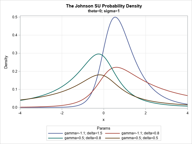
The SU distributions have relatively large kurtosis. The graph shows that the SU distribution contains a variety of unimodal curves. The blue curve (γ=–1.1, δ=1.5) and the red curve (γ=–1.1, δ=0.8) both exhibit positive skewness whereas the other curves are closer to being symmetric.

The SU distributions are useful for modeling "heavy-tailed" distributions. A random sample from a heavy-tailed distribution typically contains more observations that are far from the mean than a random normal sample of the same size. Thus you might want to use a Johnson SU distribution to model a phenomenon in which extreme events occur somewhat frequently.

The CDF and quantiles of the SU distribution

I am not aware of explicit formulas for the cumulative distribution function (CDF) and quantile function of the SU distribution. You can use numerical integration of the PDF to evaluate the cumulative distribution. You can use numerical root-finding methods to evaluate the inverse CDF (quantile) function, but it will be an expensive computation.

Fitting parameters of the SU distribution

If you have data, you can use PROC UNIVARIATE to estimate four parameters of the SU distribution that fit the data. In an earlier section, we simulated a data set for which all values are in the interval [0, 1]. The following call to PROC UNIVARIATE estimates the shape parameters for these simulated data:

proc univariate data=SU;
   histogram x / SU(theta=EST sigma=EST gamma=EST delta=EST
                    fitmethod=percentiles);
run;

The HISTOGRAM statement supports three methods for fitting the parameters from data. By default, the procedure uses the FITMETHOD=PERCENTILE method (Slifker and Shapiro, 1980) to estimate the parameters. You can also use FITMETHOD=MLE to obtain a maximum likelihood estimate or FITMETHOD=MOMENTS to estimate the parameters by matching the sample moments. For these data, I've used the percentile method. The method of moments does not provide a feasible solution for these data.

Summary

The Johnson SU distribution is a family that models unbounded distributions. It is especially useful for modeling distributions that have heavy tails. This article shows how to simulate random values from the SU distribution and how to visualize the probability density function (PDF). It also shows how to use PROC UNIVARIATE to fit parameters of the SU distribution to data.