With four parameters I can fit an elephant. With five I can make his trunk wiggle.
— John von Neumann
Ever since the dawn of statistics, researchers have searched for the Holy Grail of statistical modeling. Namely, a flexible distribution that can model any continuous univariate data. As the quote John von Neumann indicates, with enough parameters you can create a very flexible system of continuous distributions that can fit a wide range of data shapes. Some well-known flexible distributions include:
- The Pearson system of distributions (circa 1895)
- The Johnson system of distributions (1949)
- Keelin's metalog distribution (Keelin, 2016)
- Power transformations of a normal distribution: Fleishman (1978) and Headrick (2002, 2010) proposed models that use a polynomial transformation of a normal distribution. However, this system cannot model distributions that have extreme skewness and kurtosis, so it will not be considered further in this article.
A reader asked about the result of fitting a flexible distribution to data when the data distribution is a known common distribution such as normal, gamma, uniform, and so forth. Does the flexible model result in the same common distribution that generated the data? Or do you get some different distribution?
For example, suppose you simulate a large sample from the uniform distribution and then fit one of these systems to the uniformly distributed data. Is the PDF of the model the uniform distribution, or is it nonuniform?
It is an interesting question. In general, the answer is that you get a different distribution than the one that generated the data. The PDF of the model is NOT the same as the "parent" data-generating distribution. This article discusses why and provides an example for the Pearson system, the Johnson system, and the metalog system.
Moment matching for the Pearson and Johnson systems
The Pearson and Johnson systems have a similar conceptual framework: They fit moments of the data distribution. Specifically, they produce a continuous distribution that has the same skewness and kurtosis as the sample skewness and sample kurtosis in the data. (The mean and standard deviation are not used because you can always scale and translate a distribution without affecting its intrinsic shape.) Graphically, if you plot the sample skewness and kurtosis on a moment-ratio diagram, then each (skewness, kurtosis) pair corresponds to one and only one distribution in the Pearson and Johnson systems.
Consequently, the question becomes, "Which common distributions are exactly represented in the Pearson or Johnson systems?"
Fit common distributions by using the Pearson system
The Pearson system decomposes the moment-ratio diagram into 12 regions, each corresponding to a distribution, known as Type I, Type II, ..., Type XII. When you fit the model, you first determine (from the sample skewness and kurtosis) which of the 12 the regions the samples seem to be in. You then fit that chosen model to the data. Not all regions correspond to familiar distributions, but several do:
- The Type I family is the family of beta distributions.
- The Type II family is the family of symmetric beta distributions, which includes the uniform distribution as a special case.
- The Type III family contains gamma distributions.
- The Type V family contains inverse gamma distributions.
- The Type VI family contains F distributions.
- The Type VII family contains Student’s t distributions.
- The normal distribution (no type number) is a limiting case for several families.
This list is summarized by using the following image of the moment-ratio diagram, which is overlaid with the families in the Pearson system The graph is taken from the documentation of PROC SIMSYSTEM in SAS Viya.
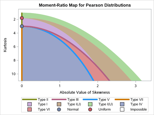
Consequently, if your data were generated by one of the distributions on this list, then when you fit a Pearson model, you have a chance to recover the true data-generating distribution. For example, if you have uniformly distributed data that has zero skewness and (full) kurtosis equal to 1.8, then you could fit the data by using a symmetric beta distribution, which would result in the uniform distribution. Conclusion: The Pearson family can fit uniformly distributed data exactly.
Fit common distributions by using the Johnson system
In contrast, the Johnson system contains only four families: The normal, the lognormal, the SB distribution (which models all bounded distributions), and the SU distribution (for unbounded distributions). Tukey's quote at the top of this article is especially applicable to the Johnson SB and SU distributions, which each contain four parameters!
Consequently, if your data are generated by the normal or lognormal distribution, you can recover the distributional form by using the Johnson system. For other familiar distributions, you cannot.
This might lead you to wonder about fitting a simple distribution such as the uniform. If the Johnson SB distribution (fitted to uniform data) does not result the uniform distribution, then what does the SB model look like? To answer that question, simulate a large data set from the U(0,1) distribution and fit the data to the SB distribution on (0,1) by using PROC UNIVARIATE, which supports the Johnson SB distribution:
/* fit a uniform distribution by using the Johnson SB distribution. What is the PDF of the model? It's NOT a constant function! */ data U; call streaminit(1); do i = 1 to 10000; u = rand("Uniform"); output; end; run; proc univariate data=U; var u; histogram u / SB(theta=0, sigma=1, fitmethod=moments) endpoints=(0 to 1 by 0.05); ods select Moments ParameterEstimates Histogram; run; |
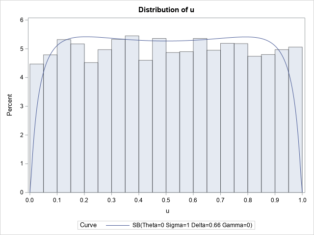
Notice that the PDF of the fitted SB distribution drops off near u=0 and u=1. This means that if you simulated samples from the fitted model, you will undersample data near the endpoints of the interval.
Fit common distributions by using the metalog system
The metalog system does not use moments or the moment-ratio diagram. Rather, it uses the empirical cumulative distribution function of the data or, more precisely, the inverse of the CDF, which is the empirical quantile function. The metalog system is based on the logistic distribution, which is the only "named" distribution that it will fit exactly.
If the metalog does not fit the uniform distribution exactly, then what does the PDF look like if you fit a metalog model to a large uniformly distributed sample? That question is a little ambiguous because the metalog system requires that you specify the order of the family, which is a parameter that determines how many component functions are used to fit the empirical quantile function.
The Appendix shows how to download the metalog package for SAS IML. Assuming that the functions in the package are stored, the following SAS IML statements fit a 5-term metalog model to the data and plot the results:
proc iml; load module=_all_; /* load the metalog function library */ use U; read all var "u"; close; /* read the data */ /* 5-term bounded metalog on [0,1] */ k = 5; MLObj = ML_CreateFromData(u, k, {0 1}); title "5-Term Metalog Model"; p = do(0,1,0.001); /* cumulative probability values */ call ML_PlotPDF(MLObj, p); /* the density function for the model */ |
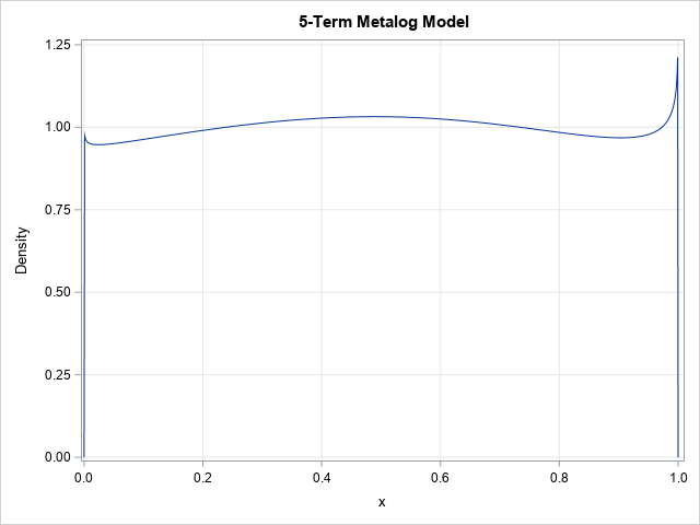
The graph is not uniform. The model has greater-than expected density in the middle of the interval and less near the endpoints. There is also a "spike" in the PDF of the model near the endpoints.
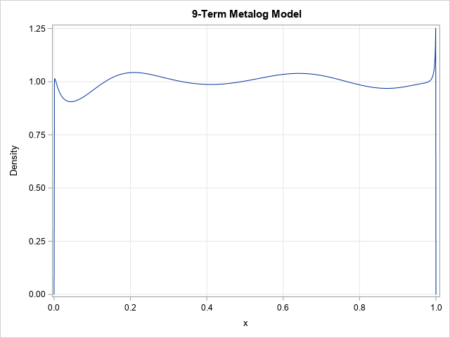
You can change the number of terms in the metalog distribution and fit the higher-order model. The result is different, but still has nonuniform probability, as shown below:
/* 9-term bounded metalog on [0,1] */ k = 9; MLObj = ML_CreateFromData(u, k, {0 1}); title "9-Term Metalog Model"; call ML_PlotPDF(MLObj, p); /* the density function for the model */ |
Summary
When you fit a flexible distribution to data that are generated by a common distribution (such as the uniform distribution), you should not expect to recover the data-generating distribution. The model will only agree with the data-generating distribution when the flexible system contains a family that is the same as the data-generating distribution.
For example, the Pearson system contains families for the beta, uniform, gamma, inverse gamma, F, t, and normal distributions. Those distributions can be represented exactly by the system. The Johnson system can fit the normal and lognormal families. The metalog system can fit the logistic distribution. All other data-generating distributions will be approximated by using the flexible distributions in the system, which have many parameters.
This article shows that a flexible model for the uniform distribution might be more complicated than you expect. That is why recommend using classical "named" distributions to model simple data distributions. Reserve the flexible families for data distributions that have complex shapes.
Appendix: Download the metalog package for SAS IML
A previous article shows how to download and use the metalog package for SAS IML software. For your convenience, the following statements were used to generate the graphs of the metalog distribution in the current article:
/*************************************/ /* metalog system: https://blogs.sas.com/content/iml/2023/03/13/metalog-sas.html Download metalog package from GitHub (do this only one time) */ /*************************************/ options dlcreatedir; %let repoPath = %sysfunc(getoption(WORK))/sas-iml-packages; /* clone repo to WORK, or use permanent libref */ /* clone repository; if repository exists, skip download */ data _null_; if fileexist("&repoPath.") then put 'Repository already exists; skipping the clone operation'; else do; put "Cloning repository 'sas-iml-packages'"; rc = gitfn_clone("https://github.com/sassoftware/sas-iml-packages/", "&repoPath." ); end; run; /*************************************/ /* Use %INCLUDE to read source code and STORE functions to current storage library */ /*************************************/ proc iml; %include "&repoPath./Metalog/ML_proc.sas"; /* each file ends with a STORE statement */ %include "&repoPath./Metalog/ML_define.sas"; quit; /*************************************/ /* now use the functions in the metalog package */ /*************************************/ proc iml; load module=_all_; /* load the metalog function library */ use U; read all var "u"; close; /* read the data */ /* 5-term bounded metalog on [0,1] */ k = 5; MLObj = ML_CreateFromData(u, k, {0 1}); title "5-Term Metalog Model"; p = do(0,1,0.001); /* cumulative probability values */ call ML_PlotPDF(MLObj, p); /* the density function for the model */ /* 9-term bounded metalog on [0,1] */ k = 9; MLObj = ML_CreateFromData(u, k, {0 1}); title "9-Term Metalog Model"; call ML_PlotPDF(MLObj, p); /* the density function for the model */ |

1 Comment
Pingback: Introducing PROC SIMSYSTEM in SAS Viya - The DO Loop