The metalog family of distributions (Keelin, Decision Analysis, 2016) is a flexible family that can model a wide range of continuous univariate data distributions when the data-generating mechanism is unknown. This article provides an overview of the metalog distributions. A subsequent article shows how to download and use a library of SAS IML functions that enable you to use the metalog distribution to model data in SAS.

The metalog distribution

There are dozens of continuous probability distributions that are commonly used to model univariate data. Examples include the normal, lognormal, Weibull, gamma, and beta distributions. (These are sometimes called "named" distributions.) Given a set of data, which distribution should you use? Ideally, you would use domain-specific knowledge to decide which distribution models the data-generating process. In practice, the process that generates the data is often unknown. Consequently, some people fit many different distributions to the data and use a goodness-of-fit statistic to choose the distribution that best fits the data.

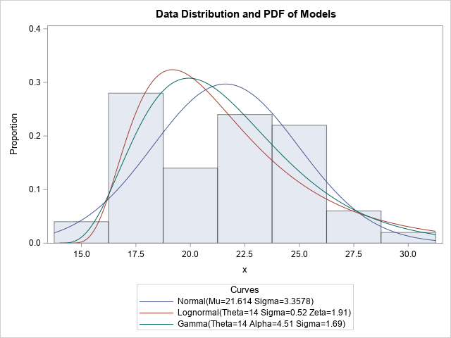
Unfortunately, this "scattershot method" is neither reliable nor principled. Furthermore, sometimes the usual well-known distributions are not sufficiently flexible to model a set of data. This is shown by the graph to the right, which shows three different distributions fit to the same data. It is not clear that one model is superior to the others.

So that modelers do not have to fit many "named" distributions and choose the best, researchers have developed flexible systems of distributions that can model a wide range of shapes. Popular systems include the following:

• The Pearson system: Karl Pearson used the normal distribution and seven other families to construct a system that can match any sample skewness and kurtosis. In SAS, you can use PROC SIMSYSTEM to fit a Pearson distribution to data.
• The Johnson system: Norman Johnson used the normal distribution, the lognormal distribution, an unbounded distribution, and a bounded distribution to match any sample skewness and kurtosis. In SAS, you can use PROC UNIVARIATE or PROC SIMSYSTEM to fit a Johnson distribution to data.
• The Fleishman system: The book Simulating Data with SAS (Wicklin, 2013) includes SAS IML modules that can fit the Fleishman system (Fleishman, 1978) to data.

The metalog system is a more recent family of distributions that can model many different shapes for bounded, semibounded, and unbounded continuous distributions. To use the metalog system, do the following:

1. Choose the type of the distribution from the four available types: unbounded, semibounded with a lower bound, semibounded with an upper bound, or bounded. This choice is often based on domain-specific knowledge of the data-generating process.
2. Choose the number of terms (k) to use in the metalog model. A small number of terms (3 ≤ k ≤ 6) results in a smooth model. A larger number of terms (k ≥ 7) can fit data distributions for which the density appears to have multiple peaks.
3. Fit the quantile function of the metalog distribution to the data. This estimates the k parameters in the model.

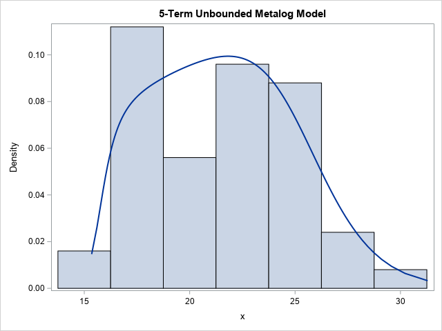
For example, the following graph shows the PDF of a 5-term unbounded metalog model overlaid on the same histogram that was previously shown. This model seems to fit the data better than the "named" distributions.

Advantages and drawbacks of using the metalog distribution

The metalog distribution has the following advantages:

• Because the metalog distribution can have many parameters, it is very flexible and can fit a wide range of shapes, including multimodal distributions.
• Keelin (2016) uses ordinary least squares (OLS) to fit the data to the quantile function of the metalog distribution. Thus, the fitting process is simple to implement.
• Because the quantile function has an explicit formula, it is simple to simulate data from the model by using the inverse CDF method of simulating data.

The metalog function has one primary disadvantage: the fitted metalog coefficients might not correspond to a valid distribution. An invalid model is called infeasible. Recall that a quantile function is always monotonically increasing as a function of the probability on the open interval (0,1). However, for an infeasible model, the quantile function is not monotonic. Equivalently, the probability density function (PDF) of the model contains nonpositive values.

Infeasibility is somewhat complicated, but one way to think about infeasibility is to think about the fact that the moments for a metalog model are related to the coefficients. If the coefficients lead to impossible moments (for example, a negative variance), then the model is infeasible.

When fitting a metalog model to data, you should always verify that the resulting model is feasible. If it is not, reduce the number of terms in the model. Some data cannot be fit when k > 2. For example, data that have one or more extreme observations often lead to an infeasible set of parameter estimates.

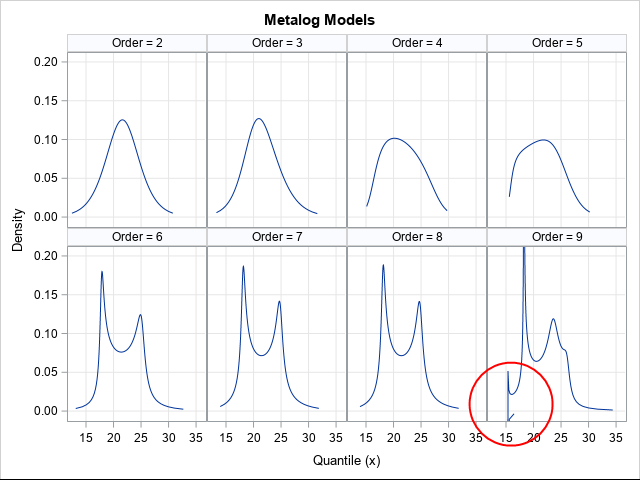
The following panel of graph shows six models for the same data. The models show increasing complexity as the number of terms increases. If you include six terms, the model becomes bimodal. However, the 9-term model is infeasible because the PDF near x=15 has a negative value, which is inside the circle in the last cell of the panel.

Definitions of the metalog distribution

Most common continuous probability distributions are parameterized on the data scale. That is, if X is a continuous random variable, then the CDF is a function that is defined on the set of outcomes for X. You can write the CDF as some increasing function p = F(x).

From the definition of a continuous CDF, you can obtain the quantile function and the PDF. The quantile function is defined as the inverse CDF: $x = F^{-1}(p)$ for p in (0,1). The PDF is defined as the derivative with respect to x of the CDF function.

Keelin (2016) specifies the definitions of the metalog quantile function and PDF function. The metalog distribution reverses the usual convention by parameterizing the quantile function as x = Q(p). From the quantile function, you can obtain the CDF, which is the inverse of the quantile function. From the CDF, you can obtain the PDF. From the quantile function, you can generate random variates. Thus, knowing the quantile function is the key to working with the metalog distribution.

The unbounded metalog distribution

When you fit an unbounded metalog model, you estimate the parameters for which the model's predicted values (p, Q(p)) are close (in a least squares sense) to the data pairs (p, x). Here, p is a vector of cumulative probabilities, x is a vector of observed data values, and Q(p) is the quantile function of a metalog distribution.

The predicted values are obtained by using a linear regression model. The unbounded model has a design matrix that uses the following basis functions:

• a vector of 1s
• a vector that contains the values logit(p) = log(p/(1-p))
• a vector that contains the values c(p) = p - 1/2

Specifically, the columns of the design matrix involve powers of the vector c(p) and interactions with the term logit(p). If M = [M1 | M2 | ... | Mk] is the design matrix, then the columns are as follows:

• M1 is a column of 1s.
• M2 is the column logit(p).
• M3 is the interaction term c(p) logit(p).
• M4 is the linear term c(p).
• M5 is the quadratic term c(p)².
• M6 is the interaction term cc(p)² logit(p).
• Additional columns are of the form c(p)^j or c(p)^j logit(p).

The following image shows the basis functions M2-M7 for the metalog regression.

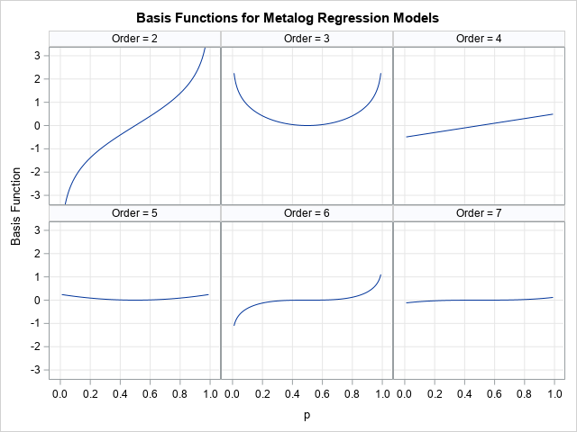
Given the design matrix, M, the least squares parameter estimates are the elements of the vector, b, which solves the matrix equations $M^\prime M b = M^\prime x$. An estimate of the quantile function is given by Q(p) = M*b. By differentiating this expression with respect to p, you can obtain a formula for the PDF for the model (Keelin, 2016, Eq. 6, p. 254).

From these equations, you can see that not every set of coefficients corresponds to an increasing quantile function. For example, when k=2, Q(p) = b1 + b2 logit(p). To be an increasing function of p, it is necessary that b2 be strictly positive.

The semibounded and bounded metalog distributions

The semibounded and bounded metalog distributions are obtained by transforming the unbounded metalog model.

The semibounded metalog distribution on the interval [L, ∞) is obtained by fitting an unbounded k-term distribution to the transformed data z = log(x-L). This gives the quantile function, Q(p), for z. The quantile function for the semibounded distribution on [L, ∞) is then defined as Q_L(p) = L + exp(Q(p)) for p in (0,1), and Q_L(0) = L.

Similarly, the quantile function for the semibounded distribution on (-∞, U) is obtained by fitting an unbounded k-term distribution to the transformed data z = log(U-x). This gives the quantile function, Q(p), for z. The quantile function for the semibounded distribution is then defined as Q_U(p) = U - exp(-Q(p)) for p in (0,1), and Q_U(1) = U.

Finally, the quantile function for the bounded metalog distribution on an interval [L, U] is obtained by fitting an unbounded k-term distribution to the transformed data z = log((x-L)/(U-x)). This gives the quantile function, Q(p), for z. The quantile function for the bounded distribution is then defined by Q_B(p) = (L + U exp(Q(p))) / (1 + exp(Q(p))) for p in (0,1), and the boundary conditions Q_B(0) = L and Q_B(1) = U.

As mentioned previously, for every distribution, you can obtain the PDF function from the quantile function.

Random variates from the metalog distribution

Recall that you can generate a random sample from any continuous probability distribution by using the inverse CDF method. You generate a random variate, u, from the uniform distribution U(0,1), then compute $x = F^{-1}(u)$, where F is the CDF function and $F^{-1}$ is the inverse CDF, which is the quantile function. You can prove that x is a random variate that is distributed according to F.

For most distributions, the inverse CDF is not known explicitly, which means that you must solve for x as the root of the nonlinear equation F(x) - u = 0. However, the metalog distribution supports direct simulation because the quantile function is defined explicitly. For the unbounded metalog distribution, you can generate random variates by generating u ~ U(0,1) and computing x = Q(u), where Q is the quantile function. The semibounded and bounded cases are treated similarly.

Summary

The metalog distribution is a flexible distribution and can fit a wide range of shapes of data distributions, including multimodal distributions. You can fit a model to data by using ordinary least squares regression. Unfortunately, not every model is feasible, which means that the model is not a valid distribution. For an infeasible model, the CDF is not monotone and the PDF is not strictly positive. Nevertheless, the metalog distribution is a powerful option for fitting data when the underlying data-generating method is unknown.

In two future articles, I show how to use a library of SAS IML functions to fit a metalog distribution to data. All the images in this article were generated in SAS by using the library.

• "Use the metalog distribution in SAS" shows how to download the Metalog package from GitHub, and how to fit metalog models in SAS.
• "Fitting a distribution to an expert's opinion" shows an application of using the metalog distribution.