Most homeowners know that large home improvement projects can take longer than you expect. Whether it's remodeling a kitchen, adding a deck, or landscaping a yard, big projects are expensive and subject to a lot of uncertainty. Factors such as weather, the availability of labor, and the supply of materials, can all contribute to uncertainty in the duration of a project.

If you ask an expert (for example, an experienced general contractor) to predict the length of time required to complete a project, he or she might respond as follows:

• 10% of the time, a project like this takes 17 work days or less.
• 50% of the time, we can complete it in 24 work days or less.
• 90% of the time, we finish the work by the 35th work day.

Whether the contractor realizes it or not, these sentences are estimating three quantiles of a continuous probability distribution for the completion of the project.

Now, if you are planning a garden party on your new deck, you don't want to schedule the party before the deck is finished. One way to predict when you can have the party is to fit a probability distribution to the contractor's estimates. But what distribution should you use? The contractor's estimates do not describe a symmetric distribution, such as the normal distribution. Without domain-specific knowledge, there is no reason to prefer one distribution over the other. Furthermore, you don't have any real data to fit the model, you have only the three estimated quantiles.

This is an excellent opportunity to use the flexible metalog family of distributions. This article shows how to convert the expert's estimates into a distribution that you can compute with and simulate data from.

Create a distribution from expert opinion

In this example, the expert predicted the quantiles (completion time) for three cumulative probabilities (10%-50%-90%). Mathematically, the expert has provided three points that are on (or near) the cumulative distribution for the completion time. Equivalently, the expert has provided three points on (or near) the quantile function. It is easy to fit a model to these values by using the metalog distribution. As discussed in a previous article, SAS supports the metalog distribution through a package of SAS IML functions that you can download from GitHub.

The following program assumes that you have downloaded and installed the metalog functions by using the instructions in the previous article or by following the instructions in Appendix A of the documentation for the metalog package, which is in the file MetalogDoc.pdf. This example uses a three-term metalog model. I assume that the project is never completed in less than 10 days, so I fit a semibounded model that has support on the interval [10, ∞). You can use the ML_CreateFromCDF function to create a metalog object from the estimates. (An estimate of this type is called a symmetric-percentile triplet (SPT) because the quantile are provided for the probabilities (α, 1/2, 1-α), where 0 < α < 1/2. In this example, α = 0.1.)

proc iml;
/* This LOAD statement assumes that the metalog functions are defined as in  Appendix A of the documentation.
   See the MetalogDoc.pdf file at https://github.com/sassoftware/sas-iml-packages/tree/main/Metalog */
load module=_all_;         
 
prob = {0.1, 0.5, 0.90};   /* cumulative probabilities; note symmetric-percentile triplet */
x    = {17,   24,  35};    /* associated quantiles */
 
order = 3;                 /* three terms in model */
bounds = {10 .};           /* support on [10, infinity) */
 
SPT = ML_CreateFromCDF(x, prob, order, bounds );  /* create model from SPT */
title "3-Term Metalog Model of Expert Opinion";
p = do(0.01, 0.99, 0.01);
run ML_PlotECDF(SPT, p);  /* graph the model CDF and the expert's estimates */

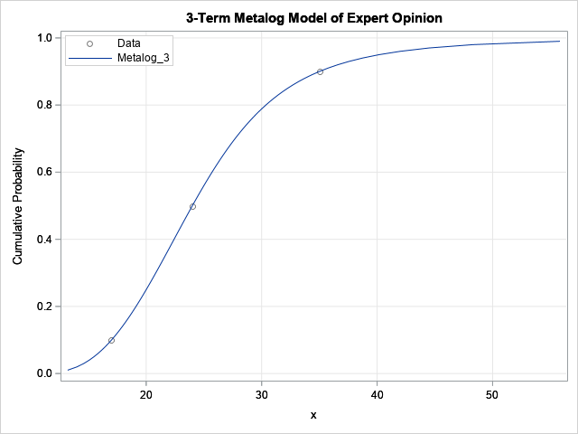
For these three data points, a three-term metalog model passes through the expert's estimates, so the model is a perfect fit. If you prefer to view the probability density for the model, you can use the ML_PlotPDF call, as follows:

title "PDF of 3-Term Metalog Model of Completion Times";
run ML_PlotPDF(SPT, p);

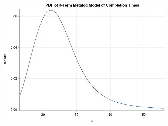
The PDF indicates the most probable duration of the project (the mode) is about 20-25 days.

The expert gave estimates for three probability values. But what if you want estimates for other probabilities? For example, let's calculate dates for which the model predicts a 95% and a 99% chance that the deck will be completed. We can get those estimates by evaluating the quantile function of the metalog model. Let's evaluate the quantile function at 0.95 and 0.99, as well as at a few other values:

/* estimates for other percentiles */
p = {0.05, 0.25, 0.75, 0.95, 0.99};
estTime = ML_Quantile(SPT, p);
print p[F=PERCENT9.] estTime[F=6.2];

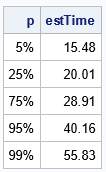
According to the model, there is a 95% chance that the project will be finished by the 40th day. There is a 99% chance that the project will be completed within 56 days. You can use those estimates to schedule a party on your new deck!

Summary

The metalog distribution can be used to construct a probability distribution from an expert's opinion. This example used three estimates for the completion of a home-improvement project. The same technique enables you to fit a metalog distribution to four, five, or more quantile estimates from an expert. The metalog model provides an easy way to convert an expert's opinion into a probability distribution that can be used for simulation and modeling.