Use the metalog distribution in SAS

A previous article describes the metalog distribution (Keelin, 2016). The metalog distribution is a flexible family of distributions that can model a wide range of shapes for data distributions. The metalog system can model bounded, semibounded, and unbounded continuous distributions. This article shows how to use the metalog distribution in SAS by downloading a library of SAS IML functions from a GitHub site.

The article contains the following sections:

An overview of the metalog library of SAS IML functions
How to download the functions from GitHub and include the functions in a program
How to use a metalog model to fit an unbounded model to data
A discussion of infeasible models

For a complete discussion of the metalog functions in SAS, see "A SAS IML Library for the Metalog Distribution" (Wicklin, 2023).

The metalog library of functions in SAS

The metalog library is a collection of SAS IML modules. The modules are object-oriented, which means that you must first construct a "metalog object," usually from raw data. The object contains information about the model. All subsequent operations are performed by passing the metalog object as an argument to functions. You can classify the functions into four categories:

Constructors create a metalog object from data. By default, the constructors fit a five-term unbounded metalog model.
Query functions enable you to query properties of the model.
Computational functions enable you to compute the PDF and quantiles of the distribution and to generate random variates.
Plotting routines create graphs of the CDF and PDF of the metalog distribution. The plotting routines are available when you use PROC IML.

Before you create a metalog object, you must choose how to model the data. There are four types of models: unbounded, semibounded with a lower bound, semibounded with an upper bound, or bounded. Then, you must decide the number of terms (k) to use in the metalog model. A small number of terms (3 ≤ k ≤ 6) results in a smooth model. A larger number of terms (k > 6) can fit multimodal data distributions, but be careful not to overfit the data by choosing k too large.

The most common way to create a metalog object is to fit a model to the empirical quantiles of the data, which estimates the k parameters in the model. For an unbounded metalog model, the quantile function is
$Q(p) = a_1 + a_2 L(p) + a_3 c(p) L(p) + a_4 c(p) + a_5 c(p)^2 + a_6 c(p)^2 L(p) + a_7 c(p)^3 + \ldots$
where L(p) = Logit(p) is the quantile function of the logistic distribution and c(p) = p – 1/2 is a linear function. You use ordinary least squares regression to fit the parameters ( $a_1, a_2, \ldots, a_k$ ) in the model.

The semibounded and bounded versions are metalog models of log-transformed variables.

If X > L, fit a metalog model to Z = log(X – L)
If L < X < U, fit a metalog model to Z = log((X – L) / (U – X))

How to download the metalog functions from GitHub

The process of downloading SAS code from a GitHub site is explained in the article, "How to use Git to share SAS programs." The process is also explained in Appendix A in the metalog documentation. The following SAS program downloads the metalog functions to the WORK libref. You could use a permanent libref, if you prefer:

/* download metalog package from GitHub */
options dlcreatedir;
%let repoPath = %sysfunc(getoption(WORK))/sas-iml-packages;  /* clone repo to WORK, or use permanent libref */
 
/* clone repository; if repository exists, skip download */
data _null_;
if fileexist("&repoPath.") then 
   put 'Repository already exists; skipping the clone operation'; 
else do;
   put "Cloning repository 'sas-iml-packages'";
   rc = gitfn_clone("https://github.com/sassoftware/sas-iml-packages/", "&repoPath." ); 
end;
run;
 
/* Use %INCLUDE to read source code and STORE functions to current storage library */
proc iml;
%include "&repoPath./Metalog/ML_proc.sas";   /* each file ends with a STORE statement */
%include "&repoPath./Metalog/ML_define.sas";
quit;

Each file ends with a STORE statement, so running the above program results in storing the metalog functions in the current storage library. The first file (ML_PROC.sas) should be included only when you are running the program in PROC IML. It contains the plotting routines. The second file (ML_define.sas) should be included in both PROC IML and the iml action.

Fit an unbounded metalog model to data

The Sashelp.heart data set contains data on patients in a heart study. The data set contains a variable (Systolic) for the systolic blood pressure of 5,209 patients. The following call to PROC SGPLOT creates a histogram of the data and overlays a kernel density estimate.

title 'Systolic Blood Pressure';
proc sgplot data=sashelp.heart;
   histogram Systolic;
   density Systolic / type=kernel;
   keylegend /location=inside;
run;

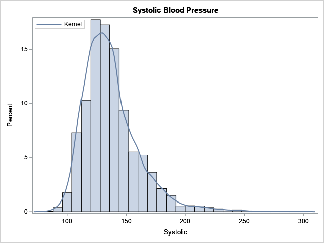
The kernel density estimate (KDE) is a nonparametric model. The histogram and the KDE indicate that the data are not normally distributed, and it is not clear whether the data can be modeled by using one of the common "named" probability distributions such as gamma or lognormal. In situations such as this, the metalog distribution can be an effective tool for modeling and simulation. The following SAS IML statements load the metalog library of functions, then fit a five-term unbounded metalog distribution to the data. After you fit the model, it is a good idea to run the ML_Summary subroutine, which displays a summary of the model and displays the parameter estimates.

proc iml;
load module=_all_;     /* load the metalog library */
use sashelp.heart;
   read all var "Systolic";
close;
 
MLObj = ML_CreateFromData(Systolic, 5);  /* 5-term unbounded model */
run ML_Summary(MLObj);

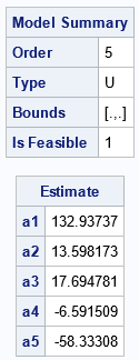
The ML_Summary subroutine displays two tables. The first table tells you that the model is a 5-term unbounded model, and it is feasible. Not every model is feasible, which is why it is important to examine the summary of the model. (Feasibility is discussed in a subsequent section.) The second table provides the parameter estimates for the model.

The MLObj variable is an object that encapsulates relevant information about the metalog model. After you create a metalog object, you can pass it to other functions to query, compute, or plot the model. For example, in PROC IML, you can use the ML_PlotECDF subroutine to show the agreement between the cumulative distribution of the model and the empirical cumulative distribution of the data, as follows:

title '5-Term Metalog Model for Systolic Blood Pressure';
run ML_PlotECDF(MLObj);

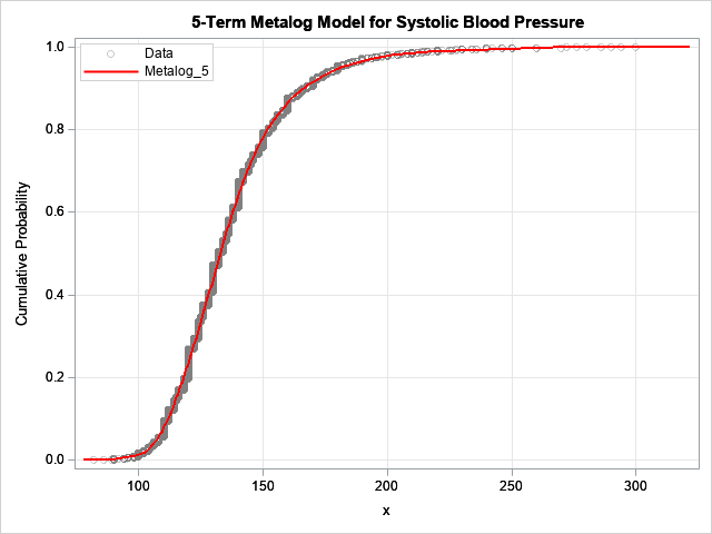
The model is fit to 5,209 observations. For this blog post, I drew the CDF of the model in red so that it would stand out. The model seems to fit the data well. If you prefer to view the density function, you can run the statement
run ML_PlotPDF(MLObj);
Again, note that the MLObj variable is passed as the first argument to the function.

One way to assess the goodness of fit is to compare the sample quantiles to the quantiles predicted by the model. You can use the ML_Quantile function to obtain the predicted quantiles, as follows:

/* estimates of quantiles */
Prob = {0.01, 0.05, 0.25, 0.5, 0.75, 0.95, 0.99};
call qntl(SampleEst, Systolic, Prob);   /* sample quantiles */
ModelEst = ML_Quantile(MLObj, Prob);    /* model quantiles */
print Prob SampleEst ModelEst;

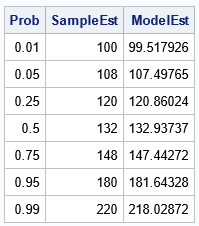
The model quantiles agree well with the sample quantiles. Note that the median estimate from the model (the 0.5 quantile) is equal to the a1 parameter estimate. This is always the case.

An advantage of the metalog model is that it has an explicit quantile function. As a consequence, it is easy to simulate from the model by using the inverse CDF method. You can use the ML_Rand function to simulate from the model, as follows:

/* simulate 500 new blood pressure values from the model */
call randseed(1234);
title 'Simulated Systolic Values';
BP = ML_Rand(MLObj, 500);
call histogram(BP);

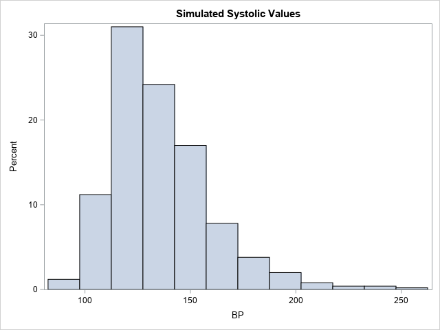
Notice that the shape of this histogram is similar to the histogram of the original data. The simulated data seem to have similar properties as the original data.

The metalog documentation provides the syntax and documentation for every public method in the library.

Infeasible metalog functions

As discussed in a previous article, not every metalog model is a valid distribution. An infeasible model is one for which the quantile function is not monotone increasing. This can happen if you have a small data set that has extreme outliers or gaps, and you attempt to fit a metalog model that has many parameters. The model will overfit the data, which results in an infeasible model.

I was unable to create an infeasible metalog model for the blood-pressure data, which has thousands of observations and no extreme observations. However, if I use only the first 20 observations, I can demonstrate an infeasible model by fitting a six-term metalog model. The following SAS IML statements create a new data vector that contains only 20 observations. A six-term metalog model is fit to those data.

/* What if we use a much smaller data set? Set N = 20. */
S = Systolic[1:20];               /* N = 20 */
MLObj = ML_CreateFromData(S, 6);  /* 6-term model */
run ML_Summary(MLObj);

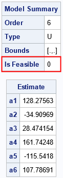
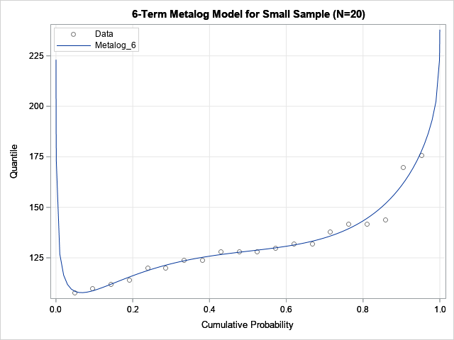
As shown by the output of the ML_Summary call, the six-term metalog model is not feasible. The following graph shows the quantile function of the model overlaid on the empirical quantiles. Notice that the quantile function of the model is not monotone increasing, which explains why the model is infeasible. If you encounter this situation in practice, Keelin (2016) suggests reducing the number of terms in the model.

Summary

This article describes how to use the metalog distribution in SAS. The metalog distribution is a flexible family that can model a wide range of distributional shapes. You can download the Metalog package from the SAS Software GitHub site. The package contains documentation and a collection of SAS IML modules. You can call the modules in a SAS IML program to fit a metalog model. After fitting the model, you can compute properties of the model and simulate data from the model. More information and examples are available in the documentation of the Metalog package.

Blogs