The tail of a probability distribution is an important notion in probability and statistics, but did you know that there is not a rigorous definition for the "tail"? The term is primarily used intuitively to mean the part of a distribution that is far from the distribution's peak or center. There are several reasons why a formal definition of "tail" is challenging:
- Where does the tail start? The tail is "far away from the mean," but how far away? For the standard normal distribution, should the tail start three standard deviations from the mean? Five?
- Not all distributions are as well-behaved as the normal distribution. The Student t distribution with 1 degree of freedom (also called the Cauchy distribution) is the classic example of a distribution that does not have a well-defined mean or variance. Consequently, it is not always possible to define the tail in terms of some number of standard deviations away from the mean or median.
- Does the uniform distribution on [0, 1] have a tail? Many people would say no. Thus not every distribution has a tail. In particular, if you want "the behavior of the tail" to describe the characteristics of the probability density function (PDF) when |x| gets large, then bounded distributions do not have tails. This example also shows that you can't merely use the 95th percentile to define the tail.
Nevertheless, some features of tails can be quantified. In particular, by using limits and asymptotic behavior you can define the notion of heavy tails. This article discusses heavy-tailed distribution and two important subclasses: the fat-tailed distributions and the long-tailed distributions.
Heavy-tailed distributions
When discussing how much mass is in the tail of a probability density function, it is convenient to use the exponential distribution as a reference. The PDF of the exponential distribution approaches zero exponentially fast. That is, the PDF looks like exp(-λx) for large values of x. Thus you can divide distributions into two categories according to the behavior of their PDFs for large values of |x|.
- Probability distribution functions that decay faster than an exponential are called thin-tailed distributions. The canonical example of a thin-tailed distribution is the normal distribution, whose PDF decreases like exp(-x2/2) for large values of |x|. A thin-tailed distribution does not have much mass in the tail, so it serves as a model for situations in which extreme events are unlikely to occur.
- Probability distribution functions that decay slower than an exponential are called heavy-tailed distributions. The canonical example of a heavy-tailed distribution is the t distribution. The tails of many heavy-tailed distributions follow a power law (like |x|–α) for large values of |x|. A heavy-tailed distribution has substantial mass in the tail, so it serves as a model for situations in which extreme events occur somewhat frequently.
Fat-tailed distributions
From a modeling perspective, fat-tailed distributions are important when extreme events must be part of the model. For example, models of claims in the home insurance industry have to account for an intense category 5 hurricane hitting the Miami area, or Superstorm Sandy flooding the New York area. Although the probability of these extreme events is small, the size of the payout is so large that these events are vital to models of insurance claims.
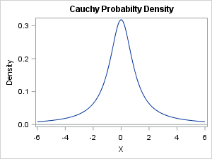
From a mathematical perspective, the most fascinating aspect of fat-tailed distributions is that the mean, variance, and other measures that describe the shape of the distribution might not be defined. You might wonder how this can be. For the symmetric Cauchy distribution, pictured at the left, it looks like the mean should be at zero. After all, the function is symmetric. However, although the Cauchy distribution has a well-defined median and mode at 0, the mean is not defined.
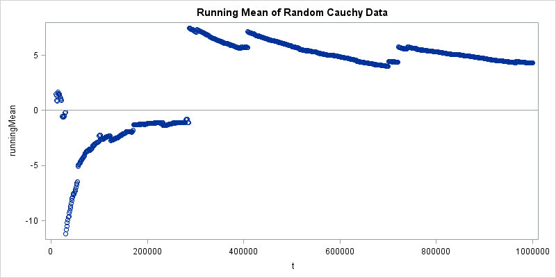
Mathematically, the problem is that a certain integral does not exist. However, a more convincing demonstration is to run a simulation that draws random values from the Cauchy distribution and computes the mean as the sample size increases. If the mean exists, then the running mean should converge to some value. But it doesn't. Instead, every so often an arbitrarily large value is generated, which causes the mean to jump by a large amount. This is shown by the following simulation and visualization in SAS software:
proc iml; call randseed(4321); N = 1e6; /* number of random draws */ x = randfun(N, "Cauchy"); /* random draws from Cauchy distribution */ RunningMean = cusum(x)/ T(1:N); /* mean for each sample size */ t = do(10000, N, 10000); /* plot the mean only for these sample sizes */ RunningMean = RunningMean[t]; title "Running Mean of Random Cauchy Data"; ods graphics / width=800px height=400px; /* size of image */ call scatter(t, RunningMean) other="refline 0 / axis=y;"; |
As an exercise, you can rerun the program for other distributions. Change the distribution family to "Normal" to see how quickly the running mean for the normal distribution converges to 0. Or change the family to "Exponential" and watch the running mean converge to 1.
Long-tailed distributions
Another kind of heavy-tailed distribution is the long-tailed distribution, which is used to model many internet-era phenomena such as the frequency distribution of book titles sold at Amazon.com or the frequency of internet search terms.
People submit billions of unique search terms to search engines. Imagine sorting all internet searches from a certain time period according to the number of times that the search term was submitted. The top-ranked terms will probably be for celebrities along with terms related to world events such as wars, natural disasters, and politics. The top-1000 search terms might account for a substantial portion of the total searches. But there are many millions of search terms that appear only a few times, or perhaps only one time. Suppose the top-1000 searches account for 10% of the total. How many search terms do you think account for 50% of the search traffic? 5,000? 10,000? The correct answer is much, much bigger! Author Chris Anderson, a former editor-in-chief at Wired magazine, says "if search were represented by a tiny lizard with a one-inch head, the tail of that lizard would stretch for 221 miles" (The Long Tail: Why the Future of Business Is Selling Less of More).
I see the same long-tailed distribution when I look at the number of views for my 500+ blog articles. The most popular 20 posts account for about 50% of the total views. But the frequency distribution of posts has a long tail, with about 180 posts getting 0.1% or more of the views, and about 300 posts getting 0.05% or more of the views. During a typical month, almost every article that I have ever written gets viewed at least once.
Attempts have been made to classify and rank distributions according to the rate of decay in their tails. For an introduction to this work, see Parzen (1979, JASA), but be sure to also read the rejoinder by John Tukey.
Summary
Although the location of the tail of a probability distribution is not rigorously defined, nevertheless a lot of research has been conducted on the asymptotic behavior of distributions. The normal and exponential distributions serve as convenient reference distributions. Distributions that have a lot of probability mass in their tails are known as heavy-tailed distributions. Two subclasses of heavy-tailed distributions are the fat-tailed distributions and the long-tailed distributions. Each is useful for modeling real-world phenomena.
Have you encountered data that exhibits a heavy tail? What was the application? How did you model the data?

5 Comments
Sure.
In my old job I modeled the transmission of sexually transmitted diseases; one variable is "number of sex partners in last year" (or last month or whatever). Another is "number of sex acts in last year". Both of these are oddly shaped, with minimum = 0, a strong peak at 1 and a long right tail. I used quantile regression, which doesn't make assumptions about the distribution of the residuals.
There are some other cases where it is generally thought that the distribution is normal, but it is not (in real samples). IQ has too many people in both far ends and has a different shaped tail on the right and left (the maximum is 200 or so, but the minimum is about 40). Weight of adults also has too many in the right tail and is not fully symmetric, but its right tail is also long (unlike that for IQ).
I very frequently encounter data which fit a normal distribution except for a few extra points in the tails. The QQ plot is basically straight in its middle section with the ends wandering away from a straight line. This is after removal of unambiguous outliers. The data are the yield of grain from small plots in series of agricultural field experiments. I know of no theoretical model which could explain this better than the normal, so I use this and advise against over-reliance on significance tests.
Pingback: Does this kurtosis make my tail look fat? - The DO Loop
Pingback: What is the coefficient of variation? - The DO Loop
Pingback: Simulate data from a generalized Gaussian distribution - The DO Loop