This article shows how to simulate a data set in SAS that satisfies a least squares regression model for continuous variables.

When you simulate to create "synthetic" (or "fake") data, you (the programmer) control the true parameter values, the form of the model, the sample size, and magnitude of the error term. You can use simulated data as a quick-and-easy way to generate an example. You can use simulation to test the performance of an algorithm on very wide or very long data sets.

The least squares regression model with continuous explanatory variables is one of the simplest regression models. The book Simulating Data with SAS describes how to simulate data from dozens of regression models. I have previously blogged about how to simulate data from a logistic regression model in SAS.

Simulate data that satisfies a linear regression model

It is useful to be able to generate data that fits a known model. Suppose you want to fit a regression model in which the response variable is a linear combination of 10 explanatory variables, plus random noise. Furthermore, suppose you don't need to use real X values; you are happy to generate random values for the explanatory variables.

The following SAS statements specify the sample size (N) and the number of explanatory variables (nCont) as macro variables. With the SAS DATA step, you can do the following:

1. Specify the model parameters, which are the regression coefficients: β₀=Intercept, β₁, β₂, β₃, .... If you know the number of explanatory variables, you can hard-code these values. The example below uses the formula β_j = (-1) ^j+1 4 / (j+1), but you can use a different formula or hard-code the parameter values.
2. Simulate the explanatory variables. In this example, the variables are independent and normally distributed. When augmented with a column that contains all 1s (to capture the model intercept), the explanatory variables form a data matrix, X.
3. Specify the error distribution, ε ∼ N(0,σ).
4. Simulate the response variable as Y = MODEL + ERROR = X β + ε.

%let N = 50;        /* Specify sample size */
%let nCont = 10;    /* Specify the number of continuous variables */
 
data SimReg1(keep= Y x:);
call streaminit(54321);              /* set the random number seed */
array x[&nCont];         /* explanatory vars are named x1-x&nCont  */
 
/* 1. Specify model coefficients. You can hard-code values such as
array beta[0:&nCont] _temporary_ (-4 2 -1.33 1 -0.8 0.67 -0.57 0.5 -0.44 0.4 -0.36);
      or you can use a formula such as the following */
array beta[0:&nCont] _temporary_;
do j = 0 to &nCont;
   beta[j] = 4 * (-1)**(j+1) / (j+1);       /* formula for beta[j]  */
end;
 
do i = 1 to &N;              /* for each observation in the sample  */
   do j = 1 to dim(x);
      x[j] = rand("Normal"); /* 2. Simulate explanatory variables   */
   end;
 
   eta = beta[0];                       /* model = intercept term   */
   do j = 1 to &nCont;
      eta = eta + beta[j] * x[j];       /*     + sum(beta[j]*x[j])  */
   end;
   epsilon = rand("Normal", 0, 1.5);    /* 3. Specify error distrib */
   Y = eta + epsilon;                   /* 4. Y = model + error     */
   output;
end;
run;

How do you know whether the simulation is correct?

After you simulate data, it is a good idea to run a regression analysis and examine the parameter estimates. For large samples, the estimates should be close to the true value of the parameters. The following call to PROC REG fits the known model to the simulated data and displays the parameter estimates, confidence intervals for the parameters, and the root mean square error (root MSE) statistic.

proc reg data=SimReg1 plots=none;
   model Y = x: / CLB;
   ods select FitStatistics ParameterEstimates;
quit;

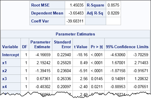
For a simple model a "large sample" does not have to be very large. Although the sample size is merely N = 50, the parameter estimates are close to the parameter values. Furthermore, the root MSE value is close to 1.5, which is the true magnitude of the error term. For this simulation, each 95% confidence interval contain the true value of the parameters, but that does not happen in general.

For more complex regression models, you might need to generate larger samples to verify that the simulation correctly generates data from the model.

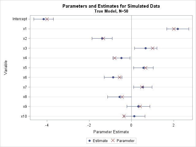
If you write the ParametereEstimates table to a SAS data set, you can create a plot that shows the parameters overlaid on a plot of the estimates and the 95% confidence limits. The plot shows that the parameters and estimates are close to each other, which should give you confidence that the simulated data are correct.

Notice that this DATA step can simulate any number of observations and any number of continuous variables. Do you want a sample that has 20, 50, or 100 variables? No problem: just change the value of the nCont macro variable! Do you want a sample that has 1000 observations? Change the value of N.

In summary, the SAS DATA step provides an easy way to simulate data from regression models in which the explanatory variables are uncorrelated and continuous. Download the complete program and modify it to your needs. For example, if you want more significant effects, use sqrt(j+1) in the denominator of the regression coefficient formula.

In a future article, I will show how to generalize this program to efficiently simulate and analyze many samples a part of a Monte Carlo simulation study.