In a previous article, I showed how to simulate data for a linear regression model with an arbitrary number of continuous explanatory variables. To keep the discussion simple, I simulated a single sample with N observations and p variables. However, to use Monte Carlo methods to approximate the sampling distribution of statistics, you need to simulate many samples from the same regression model.

This article shows how to simulate many samples efficiently. Efficient simulation is the main emphasis of my book Simulating Data with SAS. For a detailed discussion about simulating data from regression models, see chapters 11 and 12.

The SAS DATA step in my previous post contains four steps. To simulate multiple samples, put a DO loop around the steps that generate the error term and the response variable for each observation in the model. The following program modifies the previous program and creates a single data set that contains NumSamples (=100) samples. Each sample is identified by an ordinal variable named SampleID.

/* Simulate many samples from a  linear regression model */
%let N = 50;            /* N = sample size               */
%let nCont = 10;        /* p = number of continuous variables */
%let NumSamples = 100;  /* number of samples                  */
data SimReg(keep= SampleID i Y x:);
call streaminit(54321);
array x[&nCont];        /* explanatory variables are named x1-x&nCont */
 
/* 1. Specify model coefficients. You can hard-code values such as
array beta[0:&nCont] _temporary_ (-4 2 -1.33 1 -0.8 0.67 -0.57 0.5 -0.44 0.4 -0.36);
      or you can use a formula such as the following */
array beta[0:&nCont] _temporary_;
do j = 0 to &nCont;
   beta[j] = 4 * (-1)**(j+1) / (j+1);       /* formula for beta[j] */
end;
 
do i = 1 to &N;              /* for each observation in the sample */
   do j = 1 to &nCont;
      x[j] = rand("Normal"); /* 2. Simulate explanatory variables  */
   end;
 
   eta = beta[0];                       /* model = intercept term  */
   do j = 1 to &nCont;
      eta = eta + beta[j] * x[j];       /*     + sum(beta[j]*x[j]) */
   end;
 
   /* 5. simulate response for each sample */
   do SampleID = 1 to &NumSamples;      /* <== LOOP OVER SAMPLES   */
      epsilon = rand("Normal", 0, 1.5); /* 3. Specify error distrib*/
      Y = eta + epsilon;                /* 4. Y = model + error    */
      output;
   end;
end;
run;

The efficient way to analyzed simulated samples with SAS is to use BY-group processing. With By-group processing you can analyze all samples with a single procedure call. The following statements sort the data by the SampleID variable and call PROC REG to analyze all samples. The NOPRINT option ensures that the procedure does not spew out thousands of tables and graphs. (For procedures that do not support the NOPRINT option, there are other ways to turn off ODS when analyzing simulated data.) The OUTEST= option saves the parameter estimates for all samples to a SAS data set.

proc sort data=SimReg;
   by SampleID i;
run;
 
proc reg data=SimReg outest=PE NOPRINT;
   by SampleID;
   model y = x:;
quit;

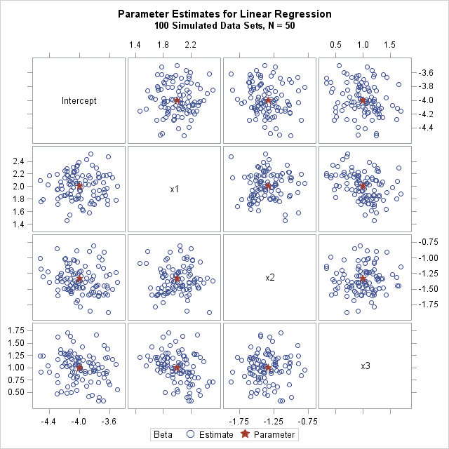
The PE data set contains NumSamples rows. Each row contains the p parameter estimates for the analysis of one simulated sample. The distribution of estimates is an approximation to the true (theoretical) sampling distribution of the statistics. The following image visualizes the joint distribution of the estimates of four regression coefficients. You can see that the distribution of the estimates appears to be multivariate normal and centered at the values of the population parameters.

You can download the SAS program that simulates the data, analyzes it, and produces the graph. The program is very efficient. For 10,000 random samples of size N=50 that contain p=10 variables, it takes about one second to run the Monte Carlo simulation and analyses.