Here's a simulation tip: When you simulate a fixed-effect generalized linear regression model, don't add a random normal error to the linear predictor. Only the response variable should be random. This tip applies to models that apply a link function to a linear predictor, including logistic regression, Poisson regression, and negative binomial regression.

Recall that a generalized linear model has three components:

1. A linear predictor η = X β, which is a linear combination of the regressors.
2. An invertible link function, g, which transforms the linear predictor to the expected value of the response variable. If μ = E(Y), then g(μ) = η or μ = g^-1(η).
3. A random component, which specifies the conditional distribution of the response variable, Y, given the values of the independent variables.

Notice that only the response variable is randomly generated. In a previous article about simulating data from a logistic regression model, I showed that the following SAS DATA step statements can be used to simulate data for a logistic regression model. The statements model a binary response variable, Y, which depends linearly on two explanatory variables X1 and X2:

   /* CORRECT way to simulate data from a logistic model with parameters (-2.7, -0.03, 0.07) */
   eta = -2.7 - 0.03*x1 + 0.07*x2;   /* linear predictor */
   mu = logistic(eta);               /* transform by inverse logit */
   y = rand("Bernoulli", mu);        /* simulate binary response with probability mu */

Notice that the randomness occurs only during the last step when you generate the response variable. Sometimes I see a simulation program in which the programmer adds a random term to the linear predictor, as follows:

   /* WRONG way to simulate logistic data. This is a latent-variable model. */
   eta = -2.7 - 0.03*x1 + 0.07*x2 + RAND("NORMAL", 0, 0.8);   /* WRONG: Leads to a misspecified model! */
   ...

Perhaps the programmer copied these statements from a simulation of a linear regression model, but it is not correct for a fixed-effect generalized linear model. When you simulate data from a generalized linear model, use the first set of statements, not the second.

Why is the second statement wrong? Because it has too much randomness. The model that generates the data includes a latent (unobserved) variable. The model you are trying to simulate is specified in a SAS regression procedure as MODEL Y = X1 X2, but the model for the latent-variable simulation (the second one) should be MODEL Y = X1 X2 X3, where X3 is the unobserved normally distributed variable.

What happens if you add a random term to the linear predictor

I haven't figured out all the mathematical ramifications of (incorrectly) adding a random term to the linear predictor prior to applying the logistic transform, but I ran a simulation that shows that the latent-variable model leads to biased parameter estimates when you fit the simulated data.

You can download the SAS program that generates data from two models: from the correct model (the first simulation steps) and from the latent-variable model (the second simulation). I generated 100 samples (each containing 5057 observations), then used PROC LOGISTIC to generate the resulting 100 sets of parameter estimates by using the statement MODEL Y = X1 X2. The results are shown in the following scatter plot matrix.

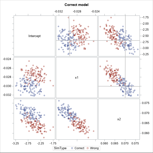
The blue markers are the parameter estimates from the correctly specified simulation. The reference lines in the upper right cells indicate the true values of the parameters in the simulation: (β₀, β₁, β₂) = (-2.7, -0.03, 0.07). You can see that the true parameter values are in the center of the cloud of blue markers, which indicates that the parameter estimates are unbiased.

In contrast, the red markers show that the parameter estimates for the misspecified latent-variable model are biased. The simulated data does not come from the model that is being fit. This simulation used 0.8 for the standard deviation of the error term in the linear predictor. If you use a smaller value, the center of the red clouds will be closer to the true parameter values. If you use a larger value, the clouds will move farther apart.

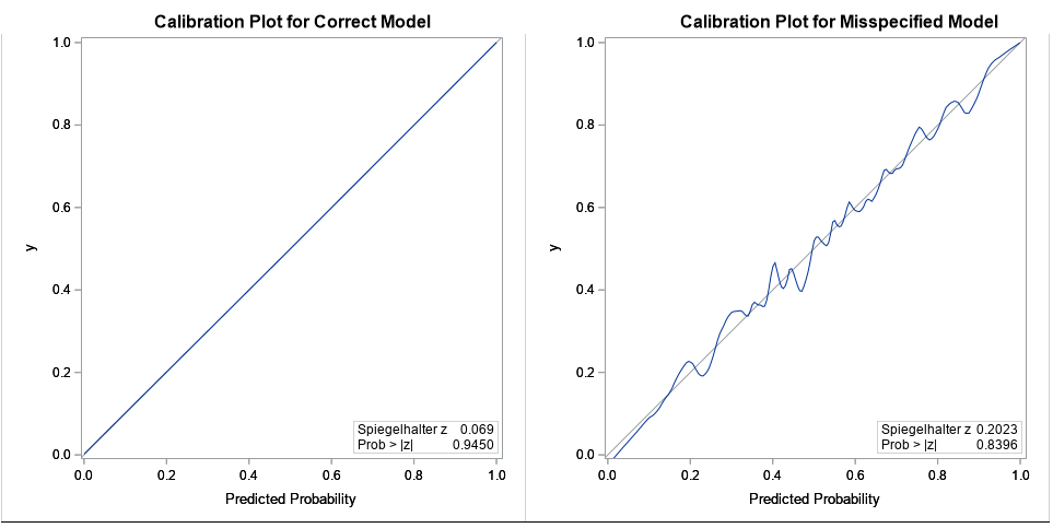
For additional evidence that the data from the second simulation does not fit the model Y = X1 X2, the following graphs show the calibration plots for a data sets from each simulation. The plot on the left shows nearly perfect calibration: This is not surprising because the data were simulated from the same model that is fitted! The plot on the right shows the calibration plot for the latent-variable model. The calibration plot shows substantial deviations from a straight line, which indicates that the model is misspecified for the second set of data.

In summary, be careful when you simulate data for a generalized fixed-effect linear model. The randomness only appears during the last step when you simulate the response variable, conditional on the linear predictor. You should not add a random term to the linear predictor.

I'll leave you with a thought that is trivial but important: You can use the framework of the generalized linear model to simulate a linear regression model. For a linear model, the link function is the identity function and the response distribution is normal. That means that a linear model can be simulated by using the following:

   /* Alternative way to simulate a linear model with parameters (-2.7, -0.03, 0.07) */
   eta = -2.7 - 0.03*x1 + 0.07*x2;   /* linear predictor */
   mu = eta;                         /* identity link function */
   y = rand("Normal", mu, 0.7);      /* simulate Y as normal response with RMSE = 0.7 */

Thus simulating a linear model fits into the framework of simulating a generalized linear model, as it should!

Download the SAS program that generates the images in this article.