Simulate data from a Poisson regression model

This article shows how to simulate data from a Poisson regression model, including how to account for an offset variable. If you are not familiar with how to run a Poisson regression in SAS, see the article "Poisson regression in SAS." A Poisson regression model is a specific type of generalized linear regression model, and I have previously showed how to simulate data from a generalized linear model.

A Poisson regression model that includes an offset

Let's begin by defining data that can be analyzed by using a Poisson regression model. The SAS documentation for PROC GENMOD includes an example that models insurance claims data. The following DATA step specifies the number of claims (Count) for a hypothetical insurance agency for three types of cars (small, medium and large) and for two age classifications (1 and 2). The data and the Poisson model are specified as follows:

data insure;
   input N Count Car$ Age;
   logN = log(N);
   Prop = Count / N;
   datalines;
500   42  Small  1
1200  37  Medium 1
100    1  Large  1
400  101  Small  2
500   73  Medium 2
300   14  Large  2
;

Because the two factors are both discrete, you can visualize the data by using a contingency table or a heat map. The following heat map visualizes the empirical proportion of claims for each combination of the CAR and AGE variable:

%let WhiteYeOrRed = (CXFFFFFF CXFFFFB2 CXFECC5C CXFD8D3C CXE31A1C);
title "Observed Counts for Claims";
proc sgplot data=insure noautolegend;
   heatmapparm x=Car y=Age colorresponse=Prop / discretex discretey 
               outline outlineattrs=(color=gray) colormodel=&WhiteYeOrRed; 
   text x=Car y=Age text=Prop; /* display the proportion in each cell */
   gradlegend;
run;

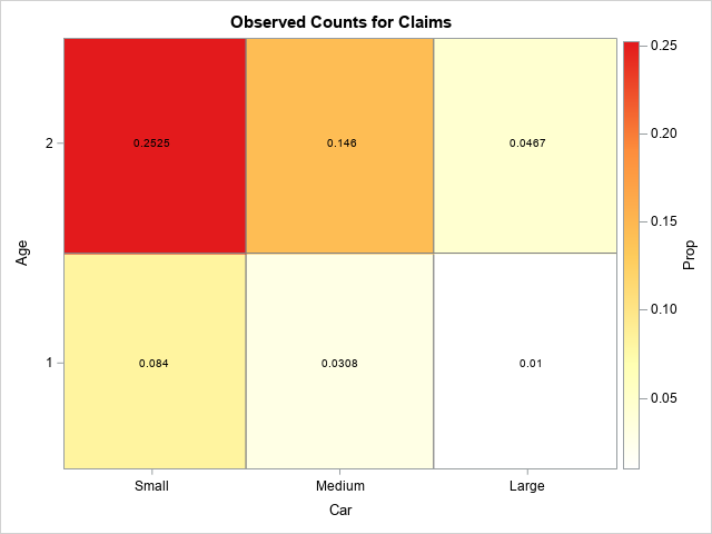
It looks like the proportions are linear in the levels of the levels of the categorical variables. For each age category, the proportions seem highest for small cars and lowest for large cars. The next section builds a Poisson regression model for these data.

Fit a Poisson regression model

You can use PROC GENMOD to fit a Poisson regression model to these data. Because the sizes of the categories are very different, it is best to model the proportion of claims rather than the raw counts of claims. To model the proportion, include an OFFSET= option on the MODEL statement in PROC GENMOD. The offset variable is the natural logarithm of a variable that indicates the size of each group. In the original data, the N variable represents the size of the groups, so the LOGN variable is used as the offset variable. The OUTPUT statement writes the linear predictor values for each observation to a variable named XBETA in the PoiModel data set,

/* Step 1: Use PROC GENMOD to fit a Poisson model to the data */
proc genmod data=insure ;
   class Age Car;
   model Count = Age Car / dist=Poisson link=log offset=logN 
                           WALDCI alpha=0.1;   /* 90% Wald CIs */
   output out=PoiModel xbeta=xbeta;
run;

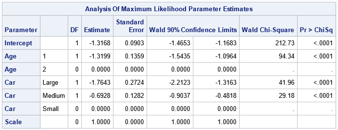
The parameter estimates table define the parameters in the Poisson regression model from which we want to simulate new data. The model is for the ratio of the variables Count/N for each group. The Poisson model fits the natural logarithm of the ratio to a linear combination of the effects in the model. These data include two categorical variables. The Age variable produces one linearly independent column in the design matrix; the Car variable produces two independent columns. Using vector notation, the model is defined by
log(Count/N) = X*β = β_Int + β₁ X_Age=1 + β₂ X_Car=Lg + β₃ X_Car=Md
or, using properties of logarithms,
log(Count) = log(N) + β_Int + β₁ X_Age=1 + β₂ X_Car=Lg + β₃ X_Car=Md
The term "log(N)" is the offset variable. The parameter estimates table shows that the best fit for these data is
log(Count) = log(N) – 1.3168 – 1.3199 X_Age=1 – 1.7643 X_Car=Lg – 0.6928 X_Car=Md

Simulate from the Poisson Model

The XBETA variable in the PoiModel data set is very useful for simulating data from the model. The documentation for the XBETA= option states that the variable contains "the estimate of the linear predictor $\mathbf{x}_i^\prime \mathbf{\beta}$ for observation i.... If there is an offset, it is included in $\mathbf{x}_i^\prime \mathbf{\beta}$ ."

You can use the XBETA variable instead of using the parameter estimates table to manually form the linear predictor. That is, in many simulation studies, you see a programming statement that looks like the following:

/* form the linear predictor, including the offset variable */
xbeta = logN -1.3168 -1.3199*(age=1) -1.7643*(car='Large') -0.6928*(car='Medium');

The XBETA output variable from PROC GENMOD contains the values of the linear combination on the right-hand side of the equation. Furthermore, the XBETA variable is computed by using the full precision of the parameter estimates, which is often more precision than copying/pasting from the values that are displayed in the ParameterEstimates table. Therefore, the following SAS DATA step simulates data from the Poisson model:

/* Step 2: Simulate many samples from the model */
/* If you use the raw data, you need to form the linear predictor yourself. 
   If you run PROC GENMOD to get the parameter estimates for real data,
   you can use the XBETA variable from the OUTPUT statement in PROC GENMOD,
   which includes the offset variable, if present.
*/
%let numSamples = 10000;
data Sim;
call streaminit(1234);
set PoiModel;  /* contains the variables N LogN Car Age and XBETA (from GENMOD) */
/* Note: the XBETA variable is from the OUTPUT statement in PROC GENMOD */
/* Apply the inverse link to XBETA (however you compute it) */
expb = exp(xbeta);
/* create a random Poisson variate; repeat for multiple simulations */
do SampleID = 1 to &numSamples;
    SimCount = rand("poisson", expb);
    SimProp = SimCount / n;   /* Optional: compute proportion from count */
    output;
end;
run;
 
/* sort by SampleID */
proc sort data=Sim;
   by SampleID;
run;

The DATA step creates 10,000 simulated samples from the Poisson model. The call to PROC SORT prepares the simulated samples for BY-group analysis, which is the most efficient way to analyze the simulated data in SAS.

Monte Carlo estimates for the Poisson model

The first step in a simulation study is to generate many independent samples. The second step is to run the Poisson model on each simulated sample and store the parameter estimates. You do not want to see all of the intermediate statistics, so turn off ODS until the analysis is complete:

/* turn off ODS: https://blogs.sas.com/content/iml/2013/05/24/turn-off-ods-for-simulations.html */
%macro ODSOff(); /* Call prior to BY-group processing */
ods graphics off; ods exclude all; ods noresults; options nonotes;
%mend;
 
%macro ODSOn(); /* Call after BY-group processing */
ods graphics on; ods exclude none; ods results; options notes;
%mend;
 
/* Step 3: run the model on each simulated sample to generate the sampling distributions */
%ODSOff;
proc genmod data=Sim;
   by SampleID;
   class age car;
   model SimCount = age car / dist=Poisson link=log offset=logN WALDCI;
   ods output ParameterEstimates=MCPE(where=(Parameter^='Scale'));  /* store statistics for each sample */
run;
%ODSOn;

The MCPE data set contains 10,000 estimates for the regression parameter.

Monte Carlo estimates of standard error and confidence intervals

There are many reasons to simulate data, but an important reason is to compute Monte Carlo estimates for the standard errors or confidence intervals for the parameters in the model. For each parameter, the MCPE data set contains 10,000 estimates. The union of the estimates approximates the sampling distribution for the statistics. The standard error of a statistic is the standard deviation of the sampling distribution. A confidence interval for a parameter is related to quantiles of the sampling distribution.

If you want to visualize, say, the sampling distribution of the Intercept term, you can create a histogram. The estimate for the Intercept of the data is -1.3168, which you can overlay on the sampling distribution, as follows:

/* Step 4: Analyze and visualize the sampling distributions to estimate standard errors,
   confidence intervals, shapes of distributions, etc. */
title "Approximate Sampling Distribution of Intercept Estimate";
proc sgplot data=MCPE;
   where Parameter='Intercept';
   histogram Estimate;
   refline -1.3168 / axis=x lineattrs=(color=red) label="Observed Intercept";
run;

The histogram shows how you would expect the Intercept estimate to vary among random samples from the specified Poisson model.

The ParameterEstimates table included estimates for the standard error and the 90% confidence interval (CI) for the parameters. For the Intercept parameter, the estimate of the standard error is 0.0903, and a 90% CI is [-1.4653, -1.1683]. These Wald estimates are based on asymptotic formulas. Let's compare them with Monte Carlo estimates from the simulation. You can use PROC MEANS to obtain the Monte Carlo estimate of the Intercept and a 90% confidence interval for the Intercept parameter, as follows:

/* compute Monte Carlo estimate of standard error and 90% Wald CI */
proc means data=MCPE mean std P5 P95 maxdec=4;
   where Parameter='Intercept';
   var Estimate;
run;

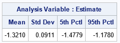
The table shows the Monte Carlo estimates. The Monte Carlo estimate for the Intercept parameter is -1.3210, which is similar to the estimate from the original data (-1.3168). The Monte Carlo estimate of the standard error is 0.0911, which you can compare to 0.0903 in the original model. Lastly, a Monte Carlo estimate of a 90% CI is [-1.4779, -1.1780], which you can compare to [-1.4653, -1.1683] in the original model. For these data and for this model, the Monte Carlo estimates agree with the asymptotic estimates to two decimal places.

You can perform a similar analysis to obtain Monte Carlo estimates for the other regression parameters. For example, the following WHERE statement selects the parameter for the Age=1 parameter:

title "Approximate Sampling Distribution of Age Estimate";
proc sgplot data=MCPE;
   where Parameter='Age' and Level1='1';
   histogram Estimate;
run;

Summary

This article shows how to simulate data from a Poisson regression model in SAS. First, you form the linear predictor (XBETA) variable. If there is an offset variable, include it in the linear predictor. PROC GENMOD generates the linear predictor automatically (and adds the offset, if necessary), but you can also specify the predictor manually, as shown in the Appendix. Then you form z = exp(XBETA) and simulate a Poisson random variate by using RAND("Poisson", z). Usually, you want to generate many random variates as part of a simulation study. You can use BY-group processing to fit the model to the simulated samples. You can use the sampling distribution of the statistics to estimate standard errors, confidence intervals, skewness, and more.

Appendix: Manual specification of the linear predictor

Although PROC GENMOD automatically creates the XBETA variable for linear models, you can also define the linear predictor manually. The following DATA step reads the values of the explanatory variables from the original data, and uses the values from the ParameterEstimates table to form XBETA .

%let numSamples = 10000;
/* for completeness, here is the same simulation from the raw data,
   which includes only the X variable at the design points */
data Sim2;
call streaminit(1234);
set insure;            /* original data; contains the variables N LogN Car and Age */
/* form the linear predictor manually */
xbeta = logN -1.31675806
        -1.76428097*(car='Large') -0.69277774*(car='Medium')
        -1.31993281*(age=1);
/* apply the inverse link */
expb = exp(xbeta);
/* create a random Poisson variate; repeat for multiple simulations */
do SampleID = 1 to &numSamples;
    SimCount = rand("poisson", expb);
    SimProp = SimCount / n;   /* Optional: compute proportion from count */
    output;
end;
run;
 
/* sort by SampleID */
proc sort data=Sim2;
   by SampleID;
run;

Blogs