There are two popular ways to express the steepness of a line or ray. The most-often used mathematical definition is from high-school math where the slope is defined as "rise over run." A second way is to report the angle of inclination to the horizontal, as introduced in basic trigonometry. If m is the rise-over-run slope of a line and θ is the angle that the line makes with the horizontal, then tan(θ) = m.

Sometimes one representation is more useful than the other. For example, I was recently studying a journal article that involved the distribution of the steepness of vectors (rays) in the plane. In this situation, representing the steepness by using angles results in a simpler description and analysis. The article discusses why angles might be a better choice for statistical computations.

An average of slopes

Statistical measures such as "the steepness of the average line" can depend on the way that you represent steepness. Because the slope and the angle are related via a nonlinear transformation, the average of the slopes is different from the average of angles.

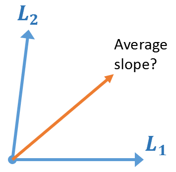
A simple thought experiment shows that the difference can be extreme. Consider two rays in the plane that are based at the origin, as illustrated in the figure to the right. The first ray is horizontal; the second is nearly vertical. Geometrically, you would expect the "average ray" to be a diagonal ray at approximately 45 degrees to the horizontal. This is confirmed algebraically if you average the angles: the average of 0 and 90 degrees is 45 degrees.

However, if you use slopes instead of angles, the averaging process does not produce the intuitive 45-degree line. Since the slope of a perfectly vertical line is undefined, let's assume that the second ray has a large finite slope, such as 10,000. If you average the nearly vertical slope and the zero slope, you obtain a slope of 5,000, which corresponds to an extremely steep line, not a 45-degree line.

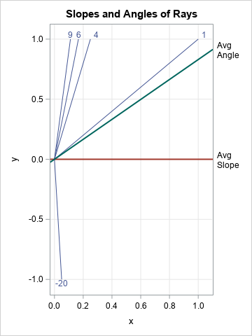
If you think a slope of 10,000 is too extreme, you can repeat the thought experiment with smaller magnitudes. Consider a set of five rays with slopes {-20, 1, 4, 6, 9}. These rays are displayed in the graph to the right and are labeled by their slopes. By inspection, the mean of these slopes is 0. But is a ray with slope 0 a good geometric estimate of the "average ray"? In contrast, if you define θ_i = ATAN(m_i), where m_i is the i_th slope, the average angle is 0.69, which is equivalent to a slope of tan(0.69) ≈ 0.83. The graph overlays the two possible "average lines," which have slopes m=0 and m=0.83. Geometrically, the average angle method seems to provide a better estimate for the steepness of a typical ray in the sample.

A uniform distribution of slopes

The previous section provides one example where using the angle of inclination to measure the steepness of a line (or ray) is preferable to using the slope formula ("rise over run"). However, the example had an outlier, and it is well known that the arithmetic mean is not robust to outliers.

For a second example, suppose you have a collection of many rays based at the origin, as in the graph below:

To the eye, the rays appear to be uniformly distributed, but in what sense? Consider the two ways to represent the steepness of each ray:

• If you use the slope to represent steepness, then the slopes are in the range (-∞, ∞) and there are two vertical rays that have undefined slopes.
• If you use the angle of inclination to represent steepness, then the angles are in the range [-π/2, π/2].

A uniform distribution is not defined on an infinite domain, so slopes are less useful for describing the distribution of lines. In contrast, a uniform distribution on [-π/2, π/2] is easy to work with. On this interval, you can work with standard statistical concepts such as mean and variance.

Notice that quantiles (including the median) and other order-based statistics might not depend on the way that the steepness is measured. For example, for an odd number of rays, the median angle and the median slope both identify the same ray. However, for an even number of rays, the median requires the arithmetic average of two measurements. As we have seen, the average of slopes can be much different than the average of angles.

Comparing a uniform distribution of slopes and angles

In the previous section, I stated that "a uniform distribution is not defined on an infinite domain." You might wonder whether that issue can be dealt with simply by limiting the slopes to a large but finite interval, such as (-1000, 1000). Let's investigate that conjecture by simulating 500 slopes from the uniform distribution on (-1000, 1000). We then graph the 500 rays that have those slopes:

/* Simulate a random sample of slopes that are uniformly distributed in (-1000, 1000).
   Most of the lines are going to fall near the Y axis and very few near the X axis. 
*/
%let Big = 1000;
data UnifSlopes;
call streaminit(1234);
do i = 1 to 500;
   slope = rand("Uniform", -&Big, &Big);  /* slope ~ U(-Big, Big) */
   x=0; y = 0;  output;        /* base of ray is (0,0) */
   x=1; y = slope*x;  output;  /* tip of ray is (1,slope) */
end;
run;
 
title "Slopes Uniform in (-&Big, &Big)";
proc sgplot data=UnifSlopes aspect=2 noautolegend;
   series x=x y=y / group=slope lineattrs=GraphData1 transparency=0.5;
   yaxis min=-1 max=1 grid;
   xaxis grid;
run;

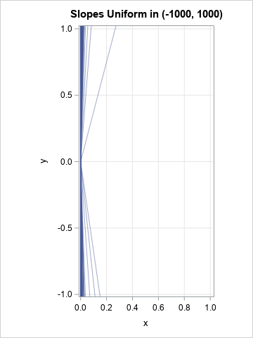
Did you expect the distribution of rays to look like this? Most of the lines are near the Y axis. Very few are near the X axis. Why? Because the probability of drawing a slope with value in an interval such as [-1, 1] is very small (1 in 1000, in this example). Therefore, it is unlikely to see a ray in a wedge near the X axis. Although the rays have uniformly distributed slopes, they do not seem to be geometrically uniform.

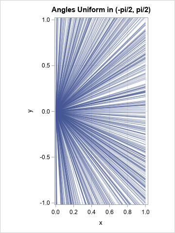
In contrast, let's simulate 500 angles uniformly in (-π/2, π/2) and plot the resulting lines:

data UnifAngles;
pi = constant('pi');
call streaminit(1234);
do i = 1 to 500;
   angle = rand("Uniform", -pi/2, pi/2);  /* angle ~ U(-pi/2, pi/2) */
   slope = tan(angle);
   x=0; y = 0;  output;        /* base of ray is (0,0) */
   x=1; y = slope*x;  output;  /* tip of ray is (1,slope) */
end;
run;
 
title "Angles Uniform in (-pi/2, pi/2)";
proc sgplot data=UnifAngles aspect=2 noautolegend;
   series x=x y=y / group=slope lineattrs=GraphData1 transparency=0.5;
   yaxis min=-1 max=1 grid;
   xaxis grid;
run;

The graph was shown in a previous section. This sample of lines have angles of inclination that are distributed uniformly. Geometrically and intuitively, this set of appears to be "more uniform" than the sample that had uniformly distributed slopes.

Summary

This article shows that there are multiple ways to measure the steepness of a set of lines. For some statistical applications, it is more useful to represent the steepness by using the angle of inclination rather than the rise-over-run definition of slope.

This article was motivated by a paper that I was reading about Passing-Bablok regression. The authors wrote an R package to accompany the paper and stated that they used angles rather than slopes to perform some computations. Initially, I did not understand why they wanted to use angles instead of slopes. Now, I do!