Compute within-group multivariate statistics and store them in a list

I recently showed how to compute within-group multivariate statistics by using the SAS/IML language. However, a principal of good software design is to encapsulate functionality and write self-contained functions that compute and return the results. What is the best way to return multiple statistics from a SAS/IML module?

A convenient way to return several statistics is to use lists. Lists were introduced in SAS/IML 14.2 and extended in SAS/IML 14.3. I have previously written about how to use lists to pass arguments into a SAS/IML module. For parallel processing in the iml action in SAS Viya, lists are an essential data structure.

This article shows two things. First, it shows how to use the UNIQUE-LOC technique to compute multivariate statistics for each group in the data. It then shows two ways to return those statistics by using SAS/IML lists. Depending on your application, one way might be more convenient to use than the other.

Returning matrices versus lists

Suppose you want to write a SAS/IML function that computes several statistics for each group in the data. If you are analyzing one variable (univariate data), the statistics are scalar. Therefore, the module can return a matrix in which the rows of the matrix represent the groups in the data and the columns represent the statistics, such as mean, median, variance, skewness, and so forth. This form of the output matches the output from PROC MEANS when you use a CLASS statement to specify the group variable.

For multivariate data, the situation becomes more complex. For example, suppose that for each group you want to compute the number of observations, the mean vector, and the covariance matrix. Although it is possible to pack all this information into a matrix, it requires a lot of bookkeeping to keep track of which row contains which statistics for which group. A simpler method is to pack the multivariate statistics into a list and return the list.

Multivariate statistics for the iris data

Fisher's iris data is often used to demonstrate ideas in multivariate statistics. The following call to PROC SGPLOT creates a scatter plot for two variables (PetalWidth and SepalLength) and uses the GROUP= option to color the observations by the levels of the Species variable. The plot also overlays 95% prediction ellipses for each group.

title "Iris Data, Colored by Species";
title2 "95% Prediction Ellipse, assuming MVN";
proc sgplot data=Sashelp.Iris;
   ellipse x=PetalWidth y=SepalWidth / group=Species outline fill transparency=0.6;
   scatter x=PetalWidth y=SepalWidth / group=Species transparency=0.2
                       markerattrs=(symbol=CircleFilled size=10) jitter;
   xaxis grid; yaxis grid;
run;

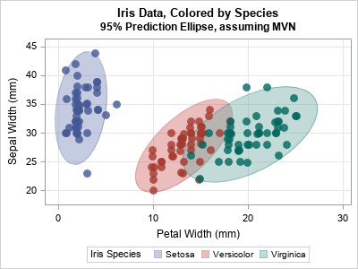
Although PROC SGPLOT computes these ellipses automatically, you might be interested in the multivariate statistics behind the ellipses. The ellipses depend on the number of observations, the mean vector, and the covariance matrix for each group. The following SAS/IML module computes these quantities for each group. The module assembles the statistics into three matrices:

The ns vector contains the number of observations. The k_th row contains the number of observations in the k_th group.
The means matrix contains the group means. The k_th row contains the mean vector for the k_th group.
The covs matrix contains the group covariance matrices. The k_th row contains the covariance matrix for the k_th group. You can use the ROWVEC function to "flatten" a matrix into a row vector. When you want to reconstruct the matrix, you can use the SHAPE function, as discussed in the article "Create an array of matrices in SAS."

These three items are packed into a list and returned by the module.

proc iml;
/* GIVEN Y and a classification variable Group that indicate group membership,
   return a list that contains:
   1. Number of observations in each group
   2. ML estimates of within-group mean
   3. ML estimate of within-group covariance 
   The k_th row of each matrix contains the statistics for the k_th group.
*/
start MLEstMVN(Y, Group);
   d = ncol(Y);
   u = unique(Group);
   G = ncol(u);
   ns    = J(G,   1, 0);           /* k_th row is number of obs in k_th group */
   means = J(G,   d, 0);           /* k_th row is mean of k_th group */
   covs  = J(G, d*d, 0) ;          /* k_th row is cov of k_th group */
 
   do k = 1 to G;
      X = Y[loc(Group=u[k]), ];    /* obs in k_th group */
      n = nrow(X);                 /* number of obs in this group */
      C = (n-1)/n * cov(X);        /* ML estimate of COV does not use the Bessel correction */
      ns[k]      = n;             
      means[k, ] = mean(X);        /* ML estimate of mean */
      covs[k, ]  = rowvec( C );    /* store COV in k_th row */
   end;
   outList = [#'n'=ns, #'mean'=means, #'cov'=Covs, #'group'=u]; /* pack into list */
   return (outList);
finish;
 
/* Example: read the iris data  */
varNames = {'PetalWidth' 'SepalWidth'};
use Sashelp.Iris;
read all var varNames into X;
read all var {'Species'};
close;
 
L = MLEstMVN(X, Species);            /* call function; return named list of results */
ns = L$'n';                          /* extract obs numbers          */
means = L$'mean';                    /* extract mean vectors         */
Covs = L$'cov';                      /* extract covariance matrix    */
lbl = L$'group';
print ns[r=lbl c='n'], 
      means[r=lbl c={'m1' 'm2'}], 
      covs[r=lbl c={C11 C12 C21 C22}];

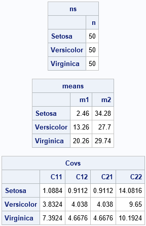
The multivariate statistics are shown. The k_th row of each matrix contains a statistic for the k_th group. The number of observations and the mean vectors are easy to understand and interpret. The covariance matrix for each group has been flattened into a row vector. You can use the SHAPE function to rearrange the row into a matrix. For example, the covariance matrix for the first group ('Setosa') can be constructed as Setosa_Cov = shape(covs[1,], 2).

An alternative: A list of lists

It can be convenient to return a list of lists that contains the statistics. Suppose you want to compute m statistics for each of G groups. The function in the previous section returned a list that contains m items and each item had G rows. (I also included an additional list item, the group levels, but that is optional.) Alternatively, you could return a list that has G sublists, where each sublist contains the m statistics for the group. This is shown in the following function, which returns the same information but organizes it in a different way.

/* Alternative: Return a list of G sublists. Each sublist has only 
   the statistics relevant to the corresponding group.    */
start MLEst2(Y, Group);
   u = unique(Group);
   G = ncol(u);
   outList = ListCreate(G);
 
   do k = 1 to G;
      X = Y[loc(Group=u[k]), ];    /* obs in k_th group */
      n = nrow(X);                 /* number of obs in k_th group */
      SL = [#'n'=n, 
            #'mean'=mean(X),        /* ML estimate of mean */
            #'cov'=(n-1)/n*cov(X)]; /* ML estimate of COV; no need to flatten */
      call ListSetItem(outList, k, SL);   /* set sublist as the k_th item */
   end;
   call ListSetName(outList, 1:G, u);     /* give a name to each sublist */
   return (outList);
finish;
 
L2 = MLEst2(X, Species);
package load ListUtil;  /* load a package to print lists */
call Struct(L2);        /* or: call ListPrint(L2);       */

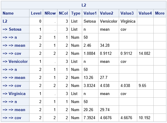
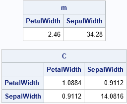
The output from the STRUCT call gives a hierarchical overview of the L2 list. The leftmost column indicates the hierarchy of the lists. The list has G=3 items, which are themselves lists. Each list has a name (the group level and m=3 items: the number of observations ('n'), the mean vector ('mean'), and the within-group MLE covariance matrix ('cov'). In this output, notice that there is no need to flatten the covariance matrix into a row vector. For some applications, this list format might be easier to work with. If you want, for example, the mean vector for the 'Setosa' group, you can access it by using the notation m = L2$'Setosa'$'mean'. Or you could extract the 'Setosa' list and access the statistics as follows:

SetosaList = L2$'Setosa';    /* get the list of statistics for the 'Setosa' group */
m = SetosaList$'mean';       /* get the mean vector */
C = SetosaList$'cov';        /* get the MLE covariance matrix */
print m[c=varNames], C[c=varNames r=varNames];

Summary

This article shows how to do two things:

How to use the UNIQUE-LOC technique to compute multivariate statistics for each group in the data.
How to return those statistics by using SAS/IML lists. Two ways to organize the output are presented. The simplest method is to stack the statistics into matrices where the k_th row represents the k_th group. You can then return a list of the matrices. The second method is to return a list of sublists, where the k_th sublist contains the statistics for the k_th list. The first method requires that you "flatten" matrices into row vectors whereas the second method does not.

Blogs