A previous article discusses the pooled variance for two or groups of univariate data. The pooled variance is often used during a t test of two independent samples. For multivariate data, the analogous concept is the pooled covariance matrix, which is an average of the sample covariance matrices of the groups. If you assume that the covariances within the groups are equal, the pooled covariance matrix is an estimate of the common covariance. This article shows how to compute and visualize a pooled covariance matrix in SAS. It explains how the pooled covariance relates to the within-group covariance matrices. It discusses a related topic, called the between-group covariance matrix.

The within-group matrix is sometimes called the within-class covariance matrix because a classification variable is used to identify the groups. Similarly, the between-group matrix is sometimes called the between-class covariance matrix.

Visualize within-group covariances

Suppose you want to analyze the covariance in the groups in Fisher's iris data (the Sashelp.Iris data set in SAS). The data set contains four numeric variables, which measure the length and width of two flower parts, the sepal and the petal. Each observation is for a flower from an iris species: Setosa, Versicolor, or Virginica. The Species variable in the data identifies observations that belong to each group, and each group has 50 observations. The following call to PROC SGPLOT creates two scatter plots and overlays prediction ellipses for two pairs of variables:

title "68% Prediction Ellipses for Iris Data";
proc sgplot data=Sashelp.Iris;
   scatter x=SepalLength y=SepalWidth / group=Species transparency=0.5;
   ellipse x=SepalLength y=SepalWidth / group=Species alpha=0.32 lineattrs=(thickness=2);
run;
proc sgplot data=Sashelp.Iris;
   scatter x=PetalLength y=PetalWidth / group=Species transparency=0.5;
   ellipse x=PetalLength y=PetalWidth / group=Species alpha=0.32 lineattrs=(thickness=2);
run;

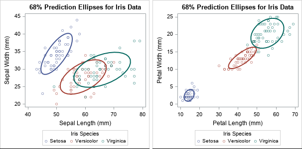
The ellipses enable you to visually investigate whether the variance of the data within the three groups appears to be the same. For these data, the answer is no because the ellipses have different shapes and sizes. Some of the prediction ellipses have major axes that are oriented more steeply than others. Some of the ellipses are small, others are relatively large.

You might wonder why the graph shows a 68% prediction ellipse for each group. Recall that prediction ellipses are a multivariate generalization of "units of standard deviation." If you assume that measurements in each group are normally distributed, 68% of random observations are within one standard deviation from the mean. So for multivariate normal data, a 68% prediction ellipse is analogous to +/-1 standard deviation from the mean.

The pooled covariance is an average of within-group covariances

The pooled covariance is used in linear discriminant analysis and other multivariate analyses. It combines (or "pools") the covariance estimates within subgroups of data. The pooled covariance is one of the methods used by Friendly and Sigal (TAS, 2020) to visualize homogeneity tests for covariance matrices.

Suppose you collect multivariate data for $k$ groups and $S_i$ is the sample covariance matrix for the $n_i$ observations within the $i$th group. If you believe that the groups have a common variance, you can estimate it by using the pooled covariance matrix, which is a weighted average of the within-group covariances:
$S_p = \Sigma_{i=1}^k (n_i-1)S_i / \Sigma_{i=1}^k (n_i - 1)$

If all groups have the same number of observations, then the formula simplifies to $\Sigma_{i=1}^k S_i / k$, which is the simple average of the matrices. If the group sizes are different, then the pooled variance is a weighted average, where larger groups receive more weight than smaller groups.

Compute the pooled covariance in SAS

In SAS, you can often compute something in two ways. The fast-and-easy way is to find a procedure that does the computation. A second way is to use the SAS/IML language to compute the answer yourself. When I compute something myself (and get the same answer as the procedure!), I increase my understanding.

Suppose you want to compute the pooled covariance matrix for the iris data. The fast-and-easy way to compute a pooled covariance matrix is to use PROC DISCRIM. The procedure supports the OUTSTAT= option, which writes many multivariate statistics to a data set, including the within-group covariance matrices, the pooled covariance matrix, and something called the between-group covariance. (It also writes analogous quantities for centered sum-of-squares and crossproduct (CSSCP) matrices and for correlation matrices.)

proc discrim data=sashelp.iris method=normal pool=yes outstat=Cov noprint;
   class Species;
   var SepalLength SepalWidth PetalLength PetalWidth;
run;
 
proc print data=Cov noobs; 
   where _TYPE_ = "PCOV";
   format _numeric_ 6.2;
   var _TYPE_ _NAME_ Sepal: Petal:;
run;

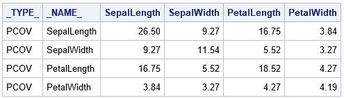
The table shows the "average" covariance matrix, where the average is across the three species of flowers.

Within-group covariance matrices

The same output data set contains the within-group and the between-group covariance matrices. The within-group matrices are easy to understand. They are the covariance matrices for the observations in each group. Accordingly, there are three such matrices for these data: one for the observations where Species="Setosa", one for Species="Versicolor", and one for Species="Virginica". The following call to PROC PRINT displays the three matrices:

proc print data=Cov noobs; 
   where _TYPE_ = "COV" and Species^=" ";
   format _numeric_ 6.2;
run;

The output is not particularly interesting, so it is not shown. The matrices are the within-group covariances that were visualized earlier by using prediction ellipses.

Visual comparison of the pooled covariance and the within-group covariance

Friendly and Sigal (2020, Figure 1) overlay the prediction ellipses for the pooled covariance on the prediction ellipses for the within-group covariances. A recreation of Figure 1 in SAS is shown below. You can use the SAS/IML language to draw prediction ellipses from covariance matrices.

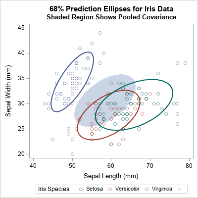
The shaded region is the prediction ellipse for these two variables in the pooled covariance matrix. It is centered at the weighted average of the group means. You can see that the pooled ellipse looks like an average of the other ellipses. This graph shows only one pair of variables, but see Figure 2 of Friendly and Sigal (2020) for a complete scatter plot matrix that compares the pooled covariance to the within-group covariance for each pair of variables.

Between-group covariance matrices

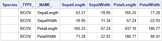
Another matrix in the PROC DISCRIM output is the so-called between-group covariance matrix. Intuitively, the between-group covariance matrix is related to the difference between the full covariance matrix of the data (where the subgroups are ignored) and the pooled covariance matrix (where the subgroups are averaged). The precise definition is given in the next section. For now, here is how to print the between-group covariance matrix from the output of PROC DISCRIM:

proc print data=Cov noobs; 
   where _TYPE_ = "BCOV";
   format _numeric_ 6.2;
run;

How to compute the pooled and between-group covariance

If I can compute a quantity "by hand," then I know that I truly understand it. Thus, I wrote a SAS/IML program that reproduces the computations made by PROC DISCRIM. The following steps are required to compute each of these matrices from first principles.

1. For each group, compute the covariance matrix (S_i) of the observations in that group.
2. Note that the quantity (n_i - 1)*S_i is the centered sum-of-squares and crossproducts (CSSCP) matrix for the group. Let M be the sum of the CSSCP matrices. The sum is the numerator for the pooled covariance.
3. Form the pooled covariance matrix as S_p = M / (N-k).
4. Let C be the CSSCP data for the full data (which is (N-1)*(Full Covariance)). The between-group covariance matrix is BCOV = (C - M) * k / (N*(k-1)).

You can use the UNIQUE-LOC trick to iterate over the data for each group. The following SAS/IML program implements these computations:

/* Compute a pooled covariance matrix when observations
   belong to k groups with sizes n1, n2, ..., nk, where n1+n2+...+nk = N
*/
proc iml;
varNames = {'SepalLength' 'SepalWidth' 'PetalLength' 'PetalWidth'};
use Sashelp.iris;
   read all var varNames into Z;
   read all var "Species" into Group;
close;
 
/* assume complete cases, otherwise remove rows with missing values */
N   = nrow(Z);
 
/* compute the within-group covariance, which is the covariance for the observations in each group */
u = unique(Group);
k = ncol(u);                /* number of groups */
p   = ncol(varNames);       /* number of variables */
M = j(p, p, 0);             /* sum of within-group CSCCP matrices */
do i = 1 to k;
   idx = loc(Group = u[i]); /* find rows for this group */
   X = Z[idx,];             /* extract obs for i_th group */
   n_i = nrow(X);           /* n_i = size of i_th group */
   S   = cov(X);            /* within-group cov */
   /* accumulate the weighted sum of within-group covariances */
   M = M + (n_i-1) * S;     /* (n_i-1)*S is centered X`*X */
end;
 
/* The pooled covariance is an average of the within-class covariance matrices. */
Sp = M / (N-k);
print Sp[L="Pooled Cov" c=varNames r=VarNames format=6.2];
 
/* The between-class CSSCP is the difference between total CSSCP and the sum of the 
   within-group CSSCPs. The SAS doc for PROC DISCRIM defines the between-class 
   covariance matrix as the between-class SSCP matrix divided by N*(k-1)/k, 
   where N is the number of observations and k is the number of classes.
*/
/* the total covariance matrix ignores the groups */
C = (N-1)*cov(Z);    
BCSSCP = C - M;               /* between = Full - Sum(Within) */
BCov = BCSSCP * k/( N*(k-1) );
print BCov[L="Between Cov" c=varNames r=VarNames format=6.2];

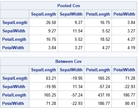
Success! The SAS/IML program shows the computations that are needed to reproduce the pooled and between-group covariance matrices. The results are the same as are produced by PROC DISCRIM.

Summary

In multivariate ANOVA, you might assume that the within-group covariance is constant across different groups in the data. The pooled covariance is an estimate of the common covariance. It is a weighted average of the sample covariances for each group, where the larger groups are weighted more heavily than smaller groups. I show how to visualize the pooled covariance by using prediction ellipses.

You can use PROC DISCRIM to compute the pooled covariance matrix and other matrices that represent within-group and between-group covariance. I also show how to compute the matrices from first principles by using the SAS/IML language. You can download the SAS program that performs the computations and creates the graphs in this article.