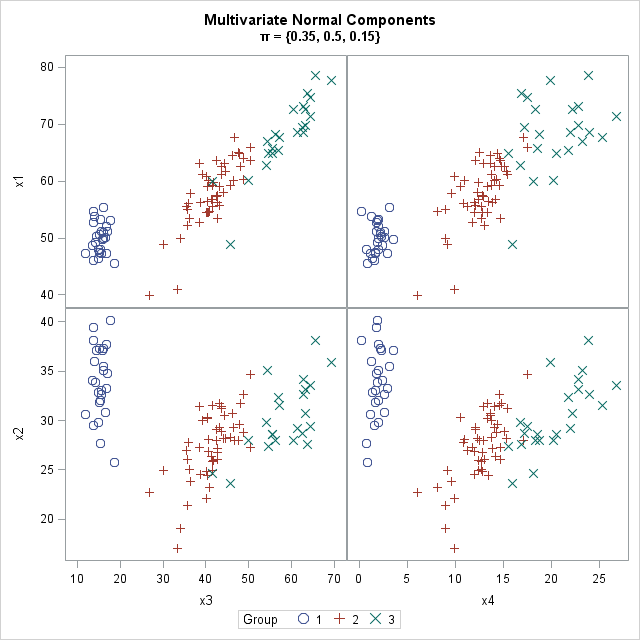
This article shows how to simulate data from a mixture of multivariate normal distributions, which is also called a Gaussian mixture. You can use this simulation to generate clustered data. The adjacent graph shows three clusters, each simulated from a four-dimensional normal distribution. Each cluster has its own within-cluster covariance, which controls the spread of the cluster and the amount overlap between clusters.

This article is based on an example in Simulating Data with SAS (Wicklin, 2013, p. 138). Previous articles have explained how to simulate from a multivariate normal distribution and how to generate a random sample from a univariate mixture distribution.

A review of mixture distributions

The graph at the top of this article shows 100 random observation from a Gaussian mixture distribution. A mixture distribution consists of K component distributions and a set of mixing probabilities that determine the probability that a random observation belongs to each component. For example, if π = {0.35, 0.5, 0.15} is a vector of mixing probabilities, then in large random samples about 35% of the observations are drawn from the first component, about 50% from the second component, and about 15% from the third component.

For a mixture of Gaussian components, you need to specify the mean vector and the covariance matrix for each component. For this example, the means and covariances are approximately the estimates from Fisher's famous iris data set, so the scatter plot matrix might look familiar to statisticians who have previously analyzed the iris data. The means of the three component distributions are μ₁ = {50, 34, 15, 2}, μ₂ = {59, 28, 43, 13}, and μ₃ = {66, 30, 56, 20}. The covariance matrices for the component distributions are shown later.

Simulate a Gaussian mixture in SAS

The SAS/IML language is the easiest way to simulate multivariate data in SAS. To simulate from a mixture of K Gaussian distributions, do the following:

1. Generate a random draw from the multinomial distribution with probability vector π. This gives the number of observations to sample from each component.
2. For each component, simulate from a multivariate normal distribution.

A technical issue is how to pass the mean vectors and covariance matrices into a module that simulates the data. If you are using SAS/IML 14.2 or beyond, you can use a list of lists (Wicklin, 2017, p. 12–14). For compatibility with older versions of SAS, the implementation in this article uses a different technique: each mean and covariance are stored as rows of a matrix. Because the covariance matrices are symmetric, Wicklin (2013) stores them in lower-triangular form. For simplicity, this article stores each 4 x 4 covariance matrix as a row in a 3 x 16 matrix.

proc iml;
/* Simulate from mixture of K mulitvariate normal distributions in dimension d.  
   OUTPUT variables:
   X  : a SampleSize x d matrix of simulated observations
   ID : a column vector that contains the component from which each obs is drawn
 
   INPUT variables:
   pi  : 1 x K vector of mixing probabilities, sum(pi)=1
   mu  : K x d matrix whose i_th row contains the mean vector for the i_th component
   Cov : K x (d**2) matrix whose i_th row contains the covariance matrix for the i_th component
*/
start SimMVNMixture(X, ID,                     /* output arguments */
                    SampleSize, pi, mu, Cov);  /* input arguments  */
   K = ncol(pi);                               /* number of components */
   d = ncol(mu);                               /* number of variables */
   X = j(SampleSize, d);                       /* output: each row is observation */
   ID = j(SampleSize, 1);                      /* ID variable */
   N = RandMultinomial(1, SampleSize, pi);     /* vector of samples sizes for components */
   b = 1;                                      /* b = beginning index for group i */
   do i = 1 to K;
      e = b + N[i] - 1;                        /* e = ending index for group i */
      ID[b:e] = i;                             /* set ID variable */
      c = shape(Cov[i,], d, d);                /* reshape Cov to square matrix */
      X[b:e, ] = RandNormal(N[i], mu[i,], c);  /* simulate i_th MVN sample */
      b = e + 1;                               /* next group starts at this index */
   end;
finish;

The SimMVNMixture routine allocates a data matrix (X) that is large enough to hold the results. It generates a vector N ={N1, N2,..., NK} to determine the number of observations that will be drawn from each component and calls the RANDNORMAL function to simulate from each Gaussian component. The scalar values b and e keep track of the beginning and ending rows of each sample from each component.

After the module is defined, you can call it for a specific set of parameters. Assume you want to generate K=3 clusters of four-dimensional data (d=4). The following statements specify the mixing probabilities for a three-component model. The mu matrix is a K x d matrix whose rows are the mean vectors for the components. The Cov matrix is a K x (d**2) matrix whose rows are the covariance matrices for the components. The following statements generate a total of 100 observations from the three-component mixture distribution:

/* specify input args; means/cov correspond to sashelp.iris data for species */
pi = {0.35 0.5 0.15};                   /* mixing probs for K=3 groups */
mu = {50 34 15  2 ,                            /* means of Group 1     */
      59 28 43 13 ,                            /* means of Group 2     */
      66 30 56 20 };                           /* means of Group 3     */
/* specify within-group covariances */
Cov = {12 10  2 1  10 14 1 1   2 1  3 1  1 1 1 1 ,   /* cov of Group 1 */
       27  9 18 6   9 10 8 4  18 8 22 7  6 4 7 4 ,   /* cov of Group 2 */
       40  9 30 5   9 10 7 5  30 7 30 5  5 5 5 8 };  /* cov of Group 3 */
/* run the simulation to generate 100 observations */
call randseed(12345);
run SimMVNMixture(X, Group, 100, pi, mu, Cov);

The call to the SimMVNMixture routine returned the simulated random sample in X, which is a 100 x d matrix. The module also returns an ID vector that identifies the component from which each observation was drawn. You can visualize the random sample by writing the data to a SAS data set and using the SGSCATTER procedure to create a paneled scatter plot, as follows:

/* save simulated data to data set */
varNames="x1":"x4";
Y = Group || X;
create Clusters from Y[c=("Group" || varNames)];  append from Y;  close;
quit;
 
ods graphics / attrpriority=none;
title "Multivariate Normal Components";
title2 "(*ESC*){unicode pi} = {0.35, 0.5, 0.15}";
proc sgscatter data=Clusters;
   compare y=(x1 x2) x=(x3 x4) / group=Group markerattrs=(Size=12);
run;

The graph is shown at the top of this article.

Although each component in this example is multivariate normal, the same technique will work for any component distributions. For example, one cluster could be multivariate normal, another multivariate t, and a third multivariate uniform.

In summary, you can create a function module in the SAS/IML language to simulate data from a mixture of Gaussian components. The RandMutinomial function returns a random vector that determines the number of observations to draw from each component. The RandNormal function generates the observations. A technical detail involves how to pass the parameters to the module. This implementation packs the parameters into matrices, but other options, such as a list of lists, are possible.