When I learn a new statistical technique, one of first things I do is to understand the limitations of the technique. This blog post shares some thoughts on modeling finite mixture models with the FMM procedure. What is a reasonable task for FMM? When are you asking too much?

I previously showed how you can use the FMM procedure to model Scrabble® scores as a mixture of three components: typical plays, triple-word scores, and penalties. That experience taught me three lessons about finite mixture models and their ability to "resolve" components that are close to each other:

• The further away the components are, the easier it is to resolve them.
• The more data you have, the better you can resolve components.
• If you can give the software hints about the components, you can resolve them better.

These lessons are not surprising, and the first two are used to determine the "power" of a statistical test. In brief, the larger the "effect" you are trying to measure, the easier it is to measure it. Similarly, larger samples have less sampling error than smaller samples, so an effect is easier to detect in larger samples. The third statement (give hints) is familiar to anyone who has used maximum likelihood estimation: a good guess for the parameter estimates can help the algorithm converge to an optimal value.

To be concrete, suppose that a population is composed of a mixture of two normal densities. Given a sample from the population, can the FMM procedure estimate the mean and variance of the underlying components? The answer depends on how far apart the two means are (relative to their variances) and how large the sample is.

The distance between components

The following figure shows the exact density for a 50/50 mixture of normal distributions, where the first component is N(0,1) and the second component is N(δ, 1). The figure shows two cases: δ=1 and 2.

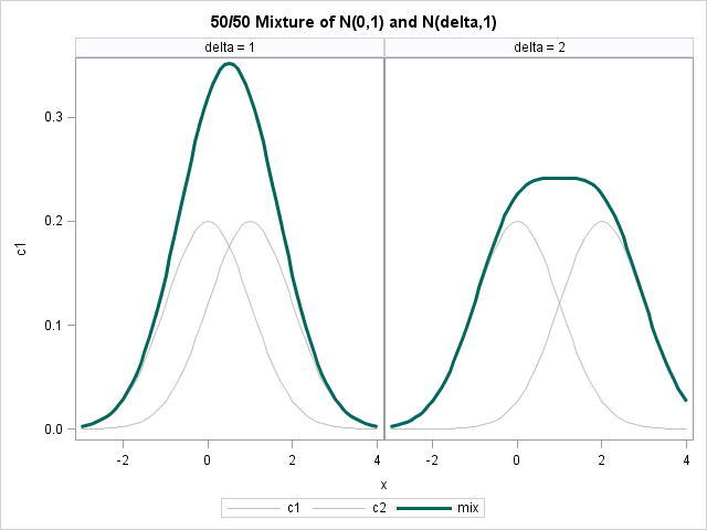
Would a human be able to look at the dark curve on the left and deduce that it is a mixture of two normal components? Unlikely. The problem is that the distance between the component densities, which is 1, is not sufficiently large relative to the variances of the components (also 1). What about the dark curve on the right? Perhaps. It depends on the person's experience with mixture models.

What happens if you generate a small number of random values (say, 100) from each probability distribution, and ask the FMM procedure to try to detect two normal components in the data? The following statements generate random values from a mixture of normals with δ=1 and δ=2, and use the FMM procedure to try to estimate the two components:

%let p = 0.5;
%let n = 100;
/* generate random values from mixture distribution */
data Sim(drop=i);
call streaminit(12345);
do delta = 1 to 2;
   do i = 1 to &n;
      c = rand("Bernoulli", &p);
      if c=0 then x = rand("normal");
      else        x = rand("normal", delta);
      output;
   end; 
end;
run;
 
/* Doesn't identify underlying components for delta=1. 
   But DOES for delta=2! */
proc fmm data=Sim;
by delta;
model x= / k=2;
run;

With only 100 points in the sample, the FMM procedure can't correctly identify the N(0,1) and N(1,1) components in the data for δ=1. However, it does correctly identify the components that are separated by a larger amount, as shown below:

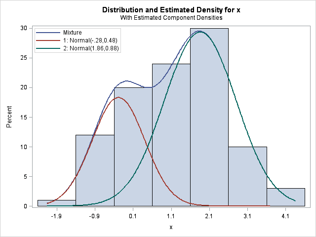
The conclusions are clear, if you have a small sample, don't expect to the FMM procedure to be able to estimate components that practically overlap.

More data = Better estimates

If you have a larger sample, the FMM procedure has more data to work with, and can detect components that do not appear distinct to the human eye. For example, if you rerun the previous example with, say, 10,000 simulated observations, then the FMM procedure has no trouble correctly identifying the N(0,1) and N(1,1) components.

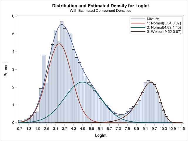
This "lesson" (more data leads to better estimates) is as old as statistics itself. Yet, when applied to the FMM procedure, you can get some pretty impressive results, such as those described in Example 37.2 in the documentation for the FMM procedure. In this example (reproduced below), two normal components and a Weibull component are identified in data that does not—to the untrained eye—look like a mixture of normals. From biological arguments, researchers knew that the density should have three components. Because the biologists had a large number of observations (141,414 of them!), the FMM procedure is able to estimate the components.

More hints = Better estimates

"Well, great," you might say, "but my sample is small and I can't collect more data. Is there any other way to coax the FMM procedure into finding relatively small effects?"

Yes, you can provide hints to the procedure. The sample and the choice of a model determines a likelihood function, which the procedure uses to estimate the parameters in the model for which the data are most likely. The likelihood function might have several local maxima, and we can use the PARMS option in the MODEL statement to provide guesses for the parameters. I used this technique to help PROC FMM estimate parameters for the three-component model of my mother's Scrabble scores.

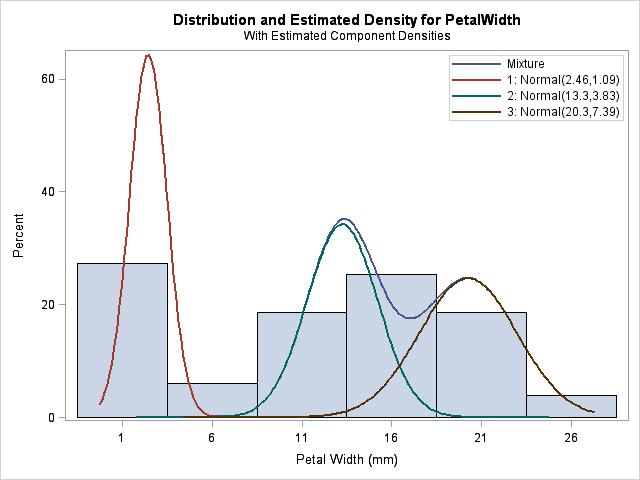
There is another important way to give a hint: you can tell the FMM procedure that one or more observations belong to particular components by using the PARTIAL= option in the PROC FMM statement. For example, it is difficult for the FMM procedure to estimate three normal components for the PetalWidth variable in the famous Fisher's iris data. Why? Because there are only 150 observations, and the means of two components are close to each other (relative to their variance). But for these data, we actually have a classification variable, Species, that identifies to which component each observation belongs. By using this extra information, the FMM procedure correctly estimates the three components:

/* give partial information about component membership */
proc fmm data=sashelp.iris partial=Species;
   class Species;
   model PetalWidth = / K=3;
run;

Is this cheating? In this case, yes, because having completely labeled data is equivalent to doing three separate density estimates, one for each species. However, the PARTIAL= option is intended to be used when you have only partial information (hence its name) about which observations are members of which component. For example, the procedure can still estimate the three components when half of the Species variable is randomly set to missing:

data iris;
set sashelp.iris;
if ranuni(1)<0.5 then Species=" "; /* set to missing */
run;

It is important to understand the limitations of any statistical modeling procedure that you use. Modeling finite mixtures with PROC FMM is no exception. If you know which tasks are reasonable and which are unrealistic, you can be more successful as a data analyst.