Sometimes a population of individuals is modeled as a combination of subpopulations. For example, if you want to model the heights of individuals, you might first model the heights of males and females separately. The height of the population can then be modeled as a combination of the male and female densities. If the subpopulations are not equally distributed, then the relative proportion of males and females in the population is used to determine the mixture density.

The population of heights is an example of a mixture distribution. The subpopulations (male and female) are the mixture components. This article describes how to sample from a mixture distribution.

Suppose that you want to model the length of time required to answer a random call received by a call center. From the data, you know that the calls typically fall into three categories. You decide to use a normal distribution to model the time required to answer each type of call, as follows:

1. Easy calls are modeled by a N(4,1) distribution (mean 4 and standard deviation 1). These account for 50% of all calls.
2. Specialized calls are modeled by a N(8,2) distribution and account for 30% of all calls.
3. Hard calls are modeled by a N(10,3) distribution and account for the remaining 20% of calls,

If you want to simulate this call center, the model suggests that you sample according to the following scheme:

• Randomly generate a category of call by using the TABLE distribution. (For details, see how to simulate categorical data.)
• After the category is determined, sample the time required to answer a call from the appropriate normal distribution.

Sampling from a mixture distribution in the DATA step

In the SAS DATA step, the following program statements us the RAND function to sample 250 calls from the call center model:

/* sample from a mixture distribution */
%let N = 250;
data Calls(drop=i);
call streaminit(12345);
array prob [3] _temporary_ (0.5 0.3 0.2);
do i = 1 to &N;
   type = rand("Table", of prob[*]);
   if type=1 then      Time = rand("Normal", 4, 1); /* easy calls */
   else if type=2 then Time = rand("Normal", 8, 2); /* specialized */
   else                Time = rand("Normal", 10, 3); /* hard */             
   output;
end;
run;

You can use the UNIVARIATE procedure to visualize the resulting sample and to estimate the population density:

proc univariate data=Calls;
ods select Histogram;
histogram Time / vscale=proportion
         kernel(lower=0 c=SJPI);              
run;

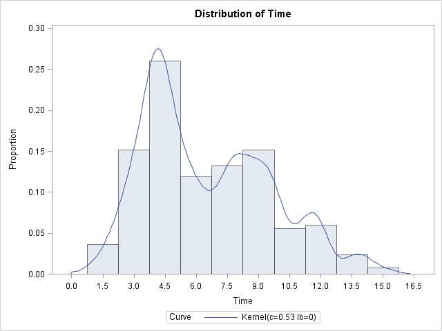
In the histogram and in the kernel density estimate, you can clearly see the high density near three minutes and near 8 minutes, which correspond to the "easy" and "specialized" calls, respectively. The density of the "hard" calls is merged with the more numerous "specialized" calls, but the "hard" calls are visible as a small bump in the density estimate.

Because a normal distribution is used to model each type of call, you can simplify the previous program by eliminating the compound IF-THEN/ELSE statements. If you put the means and standard deviations in temporary arrays, you can use the statement Time = rand("Normal", mean[type], std[type]);

Sampling from a mixture distribution in the SAS/IML Language

The following SAS/IML program samples from the same mixture distribution:

/* sample from a mixture distribution */
proc iml;
N = &N;
call randseed(12345);
prob = {0.5 0.3 0.2};
Type = j(N, 1); /* allocate vector */
call randgen(Type, "Table", prob); /* fill with 1s, 2s, and 3s */
 
mean = {4 8 10};
sd   = {1 2  3};
Time = j(N,1); /* allocate vector */
do i = 1 to ncol(prob);
   idx = loc(Type=i);
   if ncol(idx) > 0 then do;
      x = j(ncol(idx),1);
      call randgen(x, "Normal", mean[i], sd[i]);
      Time[idx] = x; /* fill with times */
   end;
end;

Notice the following features of the program:

• All of the categories are generated by a single call to the RANDGEN subroutine.
• The LOC function is used to identify the calls for each category.
• The times for each category are drawn from independent normal distributions.

The distribution of the simulated times is similar to the distribution shown in the previous histogram. Simulations like these can be used to ensure that adequate resources are in place to handle the expected number of calls for the various categories.