In my previous post, I blogged about how to sample from a finite mixture distribution. I showed how to simulate variables from populations that are composed of two or more subpopulations. Modeling a response variable as a mixture distribution is an active area of statistics, as judged by many talks on the topic at JSM 2011. When SAS 9.3 shipped, I promised to discuss my experiences with the new experimental FMM procedure, which fits finite mixture models. This article describes modeling univariate data as a mixture of normal distributions.
Initial thoughts and misconceptions
I confess: I don't know much about finite mixture models. I read some of the documentation and followed some of the examples, but I've barely begun to explore the capabilities of PROC FMM. (Thanks to my colleagues, Dave and John, for reviewing this article.)
The FMM procedure in SAS/STAT software is not a discrimination procedure. When you use the CANDISC and DISCRIM procedures, you must know the group membership for each observation in order to build a model that classifies the group membership of future observations. Similarly, most SAS regression procedures enable you to use a CLASS statement to build a model that accounts for group membership. The beauty of the FMM procedure is that you don't need this knowledge, and yet you can still build a model for response variables that are multi-modal. (You can, however, supply partial group information when you know it by using the PARTIAL option.) In my mind, I pretend that PROC FMM models the components as latent variables, since I'm familiar with that concept.
The way that the FMM procedure models a response variable reminds me of clustering procedures: You tell the FMM procedure that the response variable consists of k components, and the procedure tries to use the data to discover (and model) the group structure as part of building a regression model. This means that there are many parameters in this problem: there are the usual parameters for the regression effects, but there are also parameters that estimate the location, shape, and strength of each component.
A first example: Modeling the distribution of Scrabble® scores
As a first example, I want to see whether the FMM procedure can model a univariate distribution as a mixture of normal densities. The data are the scores for each word played in series of a Scrabble games between my mother and me.
As I wrote previously, the distribution of scores seems to have three components. Most scores are in the 12–15 point range, and correspond to standard plays. There is a small group of larger scores that correspond to triple word scores. For my mother's scores, there is a third group of small and negative scores that correspond to plays made at the end of a game. You can download the data for these Scrabble games.
For the games recorded here, my scores had few end-of-game penalties. Consequently, I assume that my scores fall into two groups. I use the FMM procedure with the K=2 option to model my scores as a mixture of two normal distributions. Notice that I specify the response variable in the MODEL statement, but do not specify any covariate effects, so this is a model for the mean of the SCORE variable:
proc fmm data=scrabble(where=(Player=2)); /* Rick's scores */ model Score = / k=2; run; |
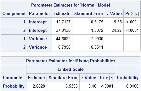
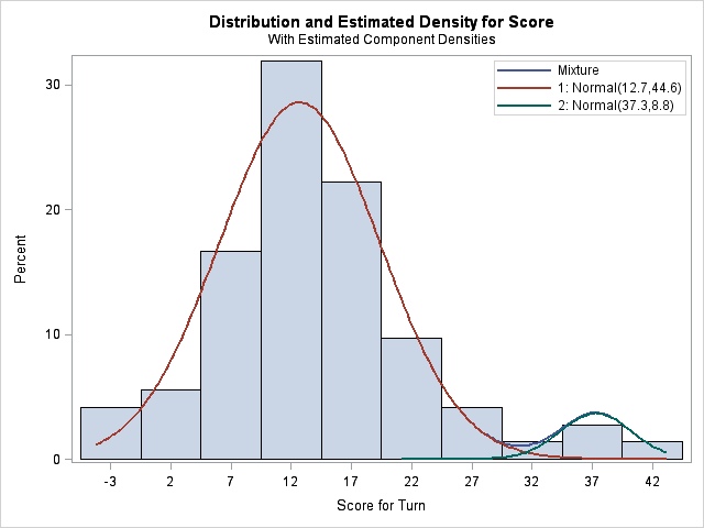
The analysis models the distribution of scores as a mixture of two normal densities. The first component has mean 12.7, which represents my average score on a "typical" word play. The variance of this distribution is 44.6, which corresponds to a standard deviation of 6.7 points per play. The second component has a mean of 37.3 and a variance of 8.8 (a standard deviation just under 3 points), and represents my triple word score plays.
The blue curve, which is almost not visible, is the overall density estimate. It is a weighted sum of the two component densities. The weights sum to unity, so there is one parameter, called the mixing parameter, that needs to be estimated by the FMM procedure in addition to the two location and scale parameters for each component. For these data, the mixing probability estimate is 2.86. This estimate is on a logit scale, which means it corresponds to a mixing probability of exp(2.86)/(exp(2.86) +exp(0)) = 0.946. This number is shown in the "Probability" column of the second table. Equivalently, the estimated PDF is 0.95*f1 + 0.05*f2, where f1 is the PDF for the first component and f2 is the PDF for the second component. These weights make sense because my mother always "steals" the triple word plays from me, which means that I have few opportunities to play a triple word score!
Now I'll try to estimate my mother's scores as a mixture of three normal densities by using the following call to the FMM procedure:
proc fmm data=scrabble(where=(Player=1)); /* Mom's scores */ model Score = / k=3; run; |
Unfortunately, this approach doesn't work very well for my mother's data. The FMM procedure converges to a set of parameters that correspond to a local maximum of the likelihood function. This solution models the data as a mixture of three distributions that are practically identical in terms of location and scale.
Fortunately, you can give "hints" to the FMM procedure by specifying starting values for the parameter estimates. The following call specifies a guess for the location and scale parameters, based on my knowledge of the game of Scrabble:
proc fmm data=scrabble(where=(Player=1)); model Score = / k=3 parms(-5 4, 13 49, 33 9); /* means: -5, 13, 33 */ run; |
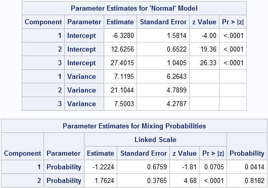
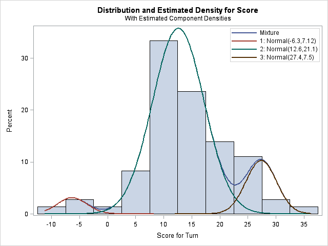
This time, the FMM procedure converges to a model that satisfies my prior beliefs. The means of the three components are at -6.3, 12.6, and 27.4. The mixing probability estimates are shown in the "Probabilities" column. They are 0.04 and 0.82, which means that the third mixing probability estimate is 0.14. Notice that the triple-word-score component for my mother accounts for 14% of the probability, whereas it accounts for only 5% of my scores.
Conclusions and gotchas
The FMM procedure did a good job of finding intuitive components for Scrabble scores. For my scores, it found two normal components such that the density of scores is a weighted sum of the components. For my mother's scores, it found three components, although I had to supply a hint. Notice that the procedure needs to estimate eight parameters in order to solve the three-component problem!
There were three lessons I learned from this exercise. The first two are "gotchas" regarding the 9.3 syntax:
- Unlike some other SAS functions, the FMM procedure represents scale in terms of the variance. If you are used to specifying the scale parameter as a standard deviation in the RAND, PDF, and CDF functions and in the UNIVARIATE and SGPLOT procedures, this convention might cause momentary confusion.
- Unlike the HISTOGRAM statement in the UNIVARIATE procedure, in which you specify all of the means followed by all of the standard deviations, the syntax of the PARMS option in the FMM procedure requires that you specify the mean and variance of each component in sequence.
The third lesson concerns the limitations of the FMM procedure. If two components of the response distribution are close to each other, then it is unreasonable to expect the FMM procedure to be able to model them as separate components. This is similar to the fact that clustering procedures have difficulties finding poorly separated clusters. I'll discuss this issue further in a future article.

18 Comments
Thanks for the great posting. It's a great tutorial for me on FMM.
I just noticed that there is a typo in the Model statement of the last sample code. The option 'parmrs' should be 'parms'.
Thanks! This is now fixed.
Pingback: The “power” of finite mixture models - The DO Loop
I am very interested in PROC FMM. I have a question here. How can I fix the means of the components? Say I already know the means of the two distributions that make up your scrabble scores (say 10 and 40). How can I specify them in the SAS code. Thanks. Great posting!
You can use the RESTRICT statement to constrain parameter values, or to fix them at a particular value.
Thanks, Rick. RESTRICT works. I have one more question if you do not mind. How to fix the parameters in Bayesian analysis for FMM? RESTRICT does not work under BAYES statement. Is there a way?
I don't know, but you can ask questions about SAS/STAT procedures at http://communities.sas.com/community/sas_statistical_procedures
Dear Rick:
A small issue I want to concern about is, which data or information in the FMM procedure can represent the value of the point at which the pdf of the two populations cross?
I don't think you can get that information directly from the FMM procedure. You might want to post your question to the SAS/STAT forum, which is for questions about how to compute statistical quantities in SAS.
Pingback: How to overlay a custom density curve on a histogram in SAS - The DO Loop
I am ok with the CDF that my model has.
But I cannot manage to translate it to an excel sheet which is the format of my deliverable.
I want to use the 3 normal distr and the weibull dist to map my x value to a accumulated probability.
For the N dist it works but the weibull with its scale and shape parameter don't work when translated to excel.
Perhaps it has to do with your comment "FMM procedure represents scale in terms of the variance" but I am lost.
the Parameterestimates output is like this:
ModelNo Label Component Parameter Effect Estimate StdErr ZValue ProbZ ILink
1 Normal 1 Intercept Intercept 59996,89206 237,1044364 253,04 0,0000
1 Normal 2 Intercept Intercept 120720,3947 293,5333585 411,27 0,0000
1 Normal 3 Intercept Intercept 180316,2952 303,1008109 594,91 0,0000
1 Normal 1 Variance Variance 2804733,195 0
1 Normal 2 Variance Variance 316366,6132 0
1 Normal 3 Variance Variance 699238,5225 0
2 Weibull 4 Intercept Intercept 11,56641767 0,016144235 716,44 0,0000 105.494,88 €
2 Weibull 4 Scale Scale Parameter 0,484896502 0,011541135
Yes, the parameterization used by PROC FMM is different from the one used by PROC UNIVARIATE and the PDF function. Try this transformation:
Dear Rick,
It is possible to retrieve the estimated intercepts using the OUTPUT statement together with the LINP option (for example: output out=want LINP).
From the retrieved values one can compute the ‘lambda’ scale parameters for different Weibull distributions as, for example, lambda_1 = exp(Linp_1) (as you also indicate above).
Do you know which parameter estimates to retrieve, using the OUTPUT statement, and from these how to compute the shape parameters ‘a’ for different Weibull distributions?
Thanks!
I wrote an article about how to interpret the regression parameters for a Weibull-distributed response. I also showed how to fit a mixture of Weibull distributions. In the second article, I show how to use the ODS OUTPUT statement to save the parameter estimates to a SAS data set. You can then automate the transformations that convert the regression estimates to estimates for the Weibull parameters.
Rick, thank you very much.
You're a data sciencist's "life saver".
To hone the learning experience, could you recommend me a reading about link functions? When it comes to logistic regression, I still can follow it, but in other context I feel lost. I'd like to understand it better.
You might want to ask that question on a social media site or on the SAS Support Communities.
Hi Rick,
Can you suggest some analysis technique, if my data is mixtureof two normals with random effects?
I haven't done it myself, but I think you can use PROC NLMIXED for this analysis. For the fixed effects, you can model Y = lambda*X1 + (1-lambda)*X2, where X1 ~ N(mu1, sigma1) and X2 ~ N(mu2, sigma2). That would be 5 parameters for the fixed effects. In situations like this, convergence might require good initial guesses.