A previous article discusses how to use SAS regression procedures to fit a two-parameter Weibull distribution in SAS. The article shows how to convert the regression output into the more familiar scale and shape parameters for the Weibull probability distribution, which are fit by using PROC UNIVARIATE.

Although PROC UNIVARIATE can fit many univariate distributions, it cannot fit a mixture of distributions. For that task, you need to use PROC FMM, which fits finite mixture models. This article discusses how to use PROC FMM to fit a mixture of two Weibull distributions and how to interpret the results. The same technique can be used to fit other mixtures of distributions. If you are going to use the parameter estimates in SAS functions such as the PDF, CDF, and RAND functions, you cannot use the regression parameters directly. You must transform them into the distribution parameters.

Simulate a mixture of Weibull data

You can use the RAND function in the SAS DATA step to simulate a mixture distribution that has two components, each drawn from a Weibull distribution. The RAND function samples from a two-parameter Weibull distribution Weib(α, β) whose density is given by
$f(x; \alpha, \beta) = \frac{\beta}{\alpha^{\beta}} (x)^{\beta -1} \exp \left(-\left(\frac{x}{\alpha}\right)^{\beta }\right)$
where α is a shape parameter and β is a scale parameter. This parameterization is used by most Base SAS functions and procedures, as well as many regression procedures in SAS. The following SAS DATA step simulates data from two Weibull distributions. The first component is sampled from Weib(α=1.5, β=0.8) and the second component is sampled from Weib(α=4, β=2). For the mixture distribution, the probability of drawing from the first distribution is 0.667 and the probability of drawing from the second distribution is 0.333.

After generating the data, you can call PROC UNIVARIATE to estimate the parameters for each component. Notice that this fits each component separately. If the parameter estimates are close to the parameter values, that is evidence that the simulation generated the data correctly.

/* sample from a mixture of two-parameter Weibull distributions */
%let N = 3000;
data Have(drop=i);
call streaminit(12345);
array prob [2] _temporary_ (0.667 0.333);
do i = 1 to &N;
   component = rand("Table", of prob[*]);
   if component=1 then
      d = rand("weibull", 1.5, 0.8);  /* C=Shape=1.5; Sigma=Scale=0.8 */
   else
      d = rand("weibull", 4,   2);    /* C=Shape=4; Sigma=Scale=2 */
   output;
end;
run;
 
proc univariate data=Have;
   class component;
   var d;
   histogram d / weibull NOCURVELEGEND;  /* fit (Sigma, C) for each component */
   ods select Histogram ParameterEstimates Moments;
   ods output ParameterEstimates = UniPE;
   inset weibull(shape scale) / pos=NE; 
run;
 
title "Weibull Estimates for Each Component";
proc print data=UniPE noobs;
   where Parameter in ('Scale', 'Shape');
   var Component Parameter Symbol Estimate;
run;

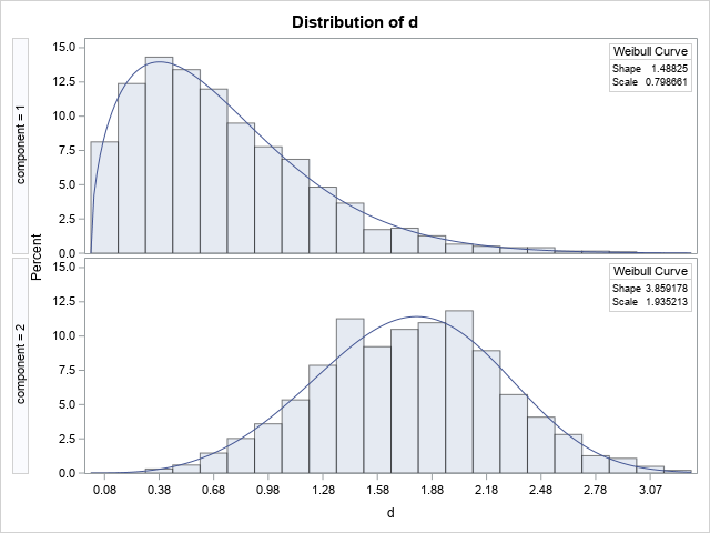
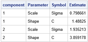
The graph shows a histogram for data in each component. PROC UNIVARIATE overlays a Weibull density on each histogram, based on the parameter estimates. The estimates for both components are close to the parameter values. The first component contains 1,970 observations, which is 65.7% of the total sample, so the estimated mixing probabilities are close to the mixing parameters. I used ODS OUTPUT and PROC PRINT to display one table that contains the parameter estimates from the two groups. PROC UNIVARIATE calls the shape parameter c and the scale parameter σ.

Fitting a finite mixture distribution

The PROC UNIVARIATE call uses the Component variable to identify the Weibull distribution to which each observation belongs. If you do not have the Component variable, is it still possible to estimate a two-component Weibull model?

The answer is yes. The FMM procedure fits statistical models for which the distribution of the response is a finite mixture of distributions. In general, the component distributions can be from different families, but this example is a homogeneous mixture, with both components from the Weibull family. When fitting a mixture model, we assume that we do not know which observations belong to which component. We must estimate the mixing probabilities and the parameters for the components. Typically, you need a lot of data and well-separated components for this effort to be successful.

The following call to PROC FMM fits a two-component Weibull model to the simulated data. As shown in a previous article, the estimates from PROC FMM are for the intercept and scale of the error term for a Weibull regression model. These estimates are different from the shape and scale parameters in the Weibull distribution. However, you can transform the regression estimates into the shape and scale parameters, as follows:

title "Weibull Estimates for Mixture";
proc fmm data=Have plots=density;
   model d = / dist=weibull link=log k=2;
   ods select ParameterEstimates MixingProbs DensityPlot;
   ods output ParameterEstimates=PE0;
run;
 
/* Add the estimates of Weibull scale and shape to the table of regression estimates.
   See https://blogs.sas.com/content/iml/2021/10/27/weibull-regression-model-sas.html */
data FMMPE;
set PE0(rename=(ILink=WeibScale));
if Parameter="Scale" then WeibShape = 1/Estimate;
else WeibShape = ._;  /* ._ is one of the 28 missing values in SAS */
run;
 
proc print data=FMMPE; 
   var Component Parameter Estimate WeibShape WeibScale;
run;

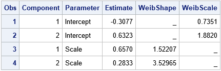
The program renames the ILink column to WeibScale. It also adds a new column (WeibShape) to the ParameterEstimates table. These two columns display the Weibull shape and scale parameter estimates for each component. Despite not knowing which observation came from which component, the procedure provides good estimates for the Weibull parameters. PROC FMM estimates the first component as Weib(α=1.52, β=0.74) and the second component as Weib(α=3.53, β=1.88). It estimates the mixing parameters for the first component as 0.,6 and the parameter for the second component as 0.4.

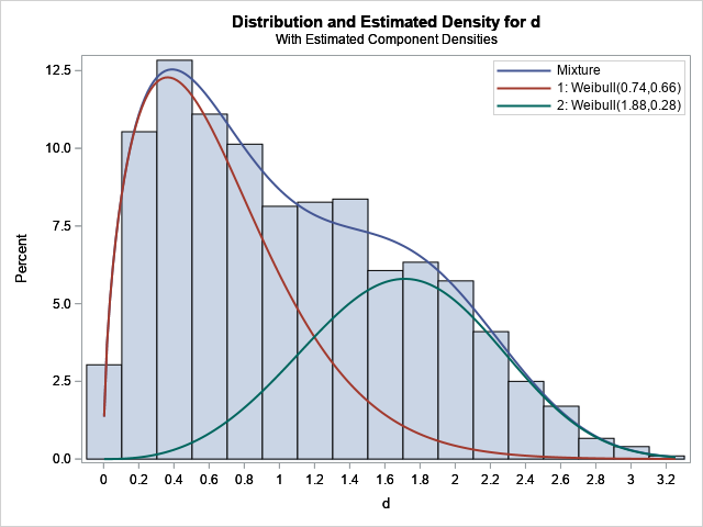
The PLOTS=DENSITY option on the PROC FMM statement produces a plot of the data and overlays the component and mixture distributions. The plot is shown below and is discussed in the next section.

The graph of the component densities

The PLOTS=DENSITY option produces a graph of the data and overlays the component and mixture distributions. In the graph, the red curve shows the density of the first Weibull component (W1(d)), the green curve shows the density of the second Weibull component (W2(d)), and the blue curve shows the density of the mixture. Technically, only the blue curve is a "true" density that integrates to unity (or 100% on a percent scale). The components are scaled densities. The integral of a component equals the mixing probability, which for these data are 0.6 and 0.4, respectively. The mixture density equals the sum of the component densities.

Look closely at the legend in the plot, which identifies the component curves by the parameter estimates. Notice, that the estimates in the legend are the REGRESSION estimates, not the shape and scale estimates for the Weibull distribution. Do not be misled by the legend. If you plot the PDF
density = PDF("Weibull", d, 0.74, 0.66); /* WRONG! */
you will NOT get the density curve for the first component. Instead, you need to convert the regression estimates into the shapes and scale parameters for the Weibull distribution. The following DATA step uses the transformed parameter estimates and demonstrates how to graph the component and mixture densities:

/* plot the Weibull component densitites and the mixture density */
data WeibComponents;
retain d1 d2;
array WeibScale[2] _temporary_ (0.7351,  1.8820);  /* =exp(Intercept) */
array WeibShape[2] _temporary_ (1.52207, 3.52965); /* =1/Scale */
array MixParm[2]   _temporary_ (0.6, 0.4);
do d = 0.01, 0.05 to 3.2 by 0.05;
   d1 = MixParm[1]*pdf("Weibull", d, WeibShape[1], WeibScale[1]); 
   d2 = MixParm[2]*pdf("Weibull", d, WeibShape[2], WeibScale[2]); 
   Component = "Mixture        "; density = d1+d2; output;
   Component = "Weib(1.52,0.74)"; density = d1;    output; 
   Component = "Weib(3.53,1.88)"; density = d2;    output; 
end;
run;
 
title "Weibull Mixture Components";
proc sgplot data=WeibComponents;
   series x=d y=density / group=Component;
   keylegend / location=inside position=NE across=1 opaque;
   xaxis values=(0 to 3.2 by 0.2) grid offsetmin=0.05 offsetmax=0.05;
   yaxis grid;
run;

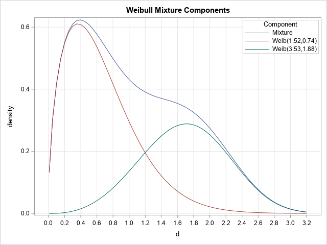
The density curves are the same, but the legend for this graph displays the shape and scale parameters for the Weibull distribution. If you want to reproduce the vertical scale (percent), you can multiply the densities by 100*h, where h=0.2 is the width of the histogram bins.

In general, be aware that the PLOTS=DENSITY option produces a graph in which the legend labels refer to the REGRESSION parameters. For example, if you use PROC FMM to fit a mixture of normal distributions, the parameter estimates in the legend are for the mean and the VARIANCE of the normal distributions. However, if you intend to use those estimates in other SAS functions (such as PDF, CDF, and RAND), you must take the square root of the variance to obtain the standard deviation.

Summary

This article uses PROC FMM to fit a mixture of two Weibull distributions. The article shows how to interpret the parameter estimates from the procedure by transforming them into the shape and scale parameters for the Weibull distribution. The article also emphasizes that if you use the PLOTS=DENSITY option produces a graph, the legend in the graph contains the regression parameters, which are not the same as the parameters that are used for the PDF, CDF, and RAND functions.