Did you know that SAS provides built-in support for working with probability distributions that are finite mixtures of normal distributions? This article shows examples of using the "NormalMix" distribution in SAS and describes a trick that enables you to easily work with distributions that have many components.

As with all probability distributions, there are four essential functions that you need to know: The PDF, CDF, QUANTILE, and RAND functions.

What is a normal mixture distribution?

A finite mixture distribution is a weighted sum of component distributions. When all of the components are normal, the distribution is called a mixture of normals. If the i_th component has parameters (μ_i, σ_i), then you can write the probability density function (PDF) of the normal mixture as
f(x) = Σ_i w_i φ(x; μ_i, σ_i)
where φ is the normal PDF and the positive constants w_i are the mixing weights. The mixing weights must sum to 1.

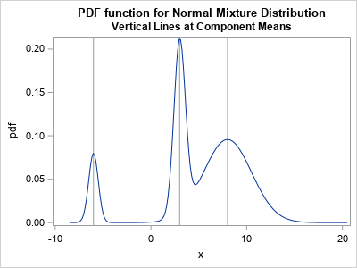
The adjacent graph shows the density function for a three-component mixture of normal distributions. The means of the components are -6, 3, and 8, respectively, and are indicated by vertical reference lines. The mixing weights are 0.1, 0.3, and 0.6. The SAS program to create the graph is in the next section.

The "NormalMix" distribution in SAS

The PDF and CDF functions in Base SAS support the "NormalMix" distribution. The syntax is a little unusual because the function needs to support an arbitrary number of components. If there are k components, the PDF and CDF functions require 3k + 3 parameters:

1. The first parameter is the name of the distribution: "NormalMix". The second parameter is the value, x, at which to evaluate the density function.
2. The third parameter is the number of component distributions, k > 1.
3. The next k parameters specify the mixing weights, w₁, w₂, ..., w_k.
4. The next k parameters specify the component means, μ₁, μ₂, ..., μ_k.
5. The next k parameters specify the component standard deviations, σ₁, σ₂, ..., σ_k.

If you are using a model that has many components, it is tedious to explicitly list every parameter in every function call. Fortunately, there is a simple trick that prevents you from having to list the parameters. You can put the parameters into arrays and use the OF operator (sometimes called the OF keyword) to reference the parameter values in the array. This is shown in the next section.

The PDF and CDF of a normal mixture

The following example demonstrates how to compute the PDF and CDF for a three-component mixture-of-normals distribution. The DATA step shows two tricks:

• The parameters (weights, means, and standard deviations) are stored in arrays. In the calls to the PDF and CDF functions, syntax such as OF w[*] enables you to specify the parameter values with minimal typing.
• A normal density is extremely tiny outside of the interval [μ - 5*σ, μ + 5*σ]. You can use this fact to compute the effective domain for the PDF and CDF functions.

/* PDF and CDF of the normal mixture distribution. This example specifies three components. */
data NormalMix;
array w[3]     _temporary_ ( 0.1, 0.3, 0.6);  /* mixing weights */ 
array mu[3]    _temporary_ (-6,   3,   8);    /* mean for each component */
array sigma[3] _temporary_ (0.5,  0.6, 2.5);  /* standard deviation for each component */
 
/* For each component, the range [mu-5*sigma, mu+5*sigma] is the effective support. */
minX = 1e308; maxX = -1e308;                  /* initialize to extreme values */
do i = 1 to dim(mu);                          /* find largest interval where density > 1E-6 */
   minX = min(minX, mu[i] - 5*sigma[i]);
   maxX = max(maxX, mu[i] + 5*sigma[i]);
end;
 
/* Visualize the functions on the effective support. Use arrays and the OF operator to
   specify the parameters. An alternative syntax is to list the arguments, as follows:
   cdf = CDF('normalmix', x, 3, 
              0.1, 0.3, 0.6,    
             -6,   3,   8,    
              0.5, 0.6, 2.5);       */
dx = (maxX - minX)/200;
do x = minX to maxX by dx;
  pdf = pdf('normalmix', x, dim(mu), of w[*], of mu[*], of sigma[*]); 
  cdf = cdf('normalmix', x, dim(mu), of w[*], of mu[*], of sigma[*]); 
  output;
end;
keep x pdf cdf;
run;

As shown in the program, the OF operator greatly simplifies and clarifies the function calls. The alternative syntax, which is shown in the comments, is unwieldy.

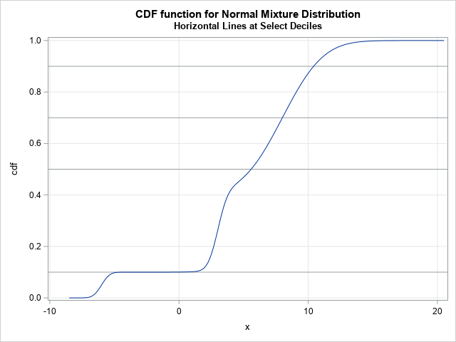
The following statements create graphs of the PDF and CDF functions. The PDF function is shown at the top of this article. The CDF function, along with a few reference lines, is shown below.

title "PDF function for Normal Mixture Distribution";
title2 "Vertical Lines at Component Means";
proc sgplot data=NormalMix;
   refline -6 3 8 / axis=x;
   series x=x y=pdf;
run;
 
title "CDF function for Normal Mixture Distribution";
proc sgplot data=NormalMix;
   xaxis grid; yaxis min=0 grid; 
   refline 0.1 0.5 0.7 0.9;
   series x=x y=cdf;
run;

The quantiles of a normal mixture

The quantile function for a continuous distribution is the inverse of the CDF distribution. The graph of the CDF function for a mixture of normals can have flat regions when the component means are far apart relative to their standard deviations. Technically, these regions are not completely flat because the normal distribution has infinite support, but computationally they can be very flat. Because finding a quantile is equivalent to finding the root of a shifted CDF, you might encounter computational problems if you try to compute the quantile that corresponds to an extremely flat region, such as the 0.1 quantile in the previous graph.

The following DATA step computes the 0.1, 0.5, 0.7, and 0.9 quantiles for the normal mixture distribution. Notice that you can use arrays and the OF operator for the QUANTILE function:

data Q;
array w[3]     _temporary_ ( 0.1, 0.3, 0.6);  /* mixing weights */ 
array mu[3]    _temporary_ (-6,   3,   8);    /* mean for each component */
array sigma[3] _temporary_ (0.5,  0.6, 2.5);  /* standard deviation for each component */
 
array p[4] (0.1, 0.5, 0.7, 0.9);  /* find quantiles for these probabilities */
do i = 1 to dim(p);
   prob = p[i];
   qntl = quantile('normalmix', prob, dim(mu), of w[*], of mu[*], of sigma[*]); 
   output;
end;
keep qntl prob;
run;
 
proc print; run;

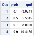
The table tells you that 10% of the density of the normal mixture is less than x=-3.824. That is essentially the result of the first component, which has weight 0.1 and therefore is responsible for 10% of the total density. Half of the density is less than x=5.58. Fully 70% of the density lies to the left of x=8, which is the mean of the third component. That result makes sense when you look at the mixing weights.

Random values from a normal mixture

The RAND function does not explicitly support the "NormalMix" distribution. However, as I have shown in a previous article, you can simulate from an arbitrary mixture of distributions by using the "Table" distribution in conjunction with the component distributions. For the three-component mixture distribution, the following DATA step simulates a random sample:

/* random sample from a mixture distribution */
%let N = 1000;
data RandMix(drop=i);
call streaminit(12345);
array w[3]     _temporary_ ( 0.1, 0.3, 0.6);  /* mixing weights */ 
array mu[3]    _temporary_ (-6,   3,   8);    /* mean for each component */
array sigma[3] _temporary_ (0.5,  0.6, 2.5);  /* standard deviation for each component */
do obsNum = 1 to &N;
   i = rand("Table", of w[*]);                /* choose the component by using the mixing weights */
   x = rand("Normal", mu[i], sigma[i]);       /* sample from that component */
   output;
end;
run;
 
title "Random Sample for Normal Mixture Distribution";
proc sgplot data=RandMix;
   histogram x;
   refline -6 3 8 / axis=x;   /* means of component distributions */
run;

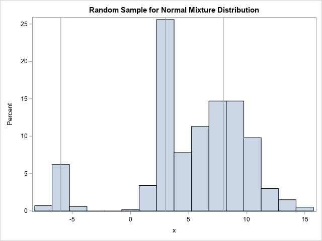
The histogram of a random sample looks similar to the graph of the PDF function, as it should.

In summary, SAS provides built-in support for working with the density (PDF), cumulative probability (CDF), and quantiles (QUANTILE) of a normal mixture distribution. You can use arrays and the OF operator to call these Base SAS functions without having to list every parameter. Although the RAND function does not natively support the "NormalMix" distribution, you can use the "Table" distribution to select a component according to the mixing weights and use the RAND("Normal") function to simulate from the selected normal component.