A statistical programmer asked how to simulate event-trials data for groups. The subjects in each group have a different probability of experiencing the event. This article describes one way to simulate this scenario. The simulation is similar to simulating from a mixture distribution. This article also shows three different ways to visualize the results of the simulation.
Modeling the data-generation process
A simulation is supposed to reproduce a data-generation process. Typically, a simulation is based on some real data. You (the programmer) need to ensure that the simulation reflects how the real data are generated. For example, there are often differences between simulating a designed experiment or simulating an observational study:
- In a designed experiment, the number of subjects in each group is determined by the researcher. For example, a researcher might choose 100 subjects, 50 men and 50 women. If so, each simulated data sample should also contain 50 males and 50 females.
- In an observational study, the number of subjects in each group is a random variable that is based on the proportion of the population in each group. For example, a researcher might choose 100 subjects at random. In the data, there might be 53 men and 47 women, but that split is the result of random chance. Each simulated data sample should generate the number of males and females according to a random binomial variable. Some samples might have a 52:48 split, others a 49:51 split, and so on. In general, the group sizes are simulated from a multinomial distribution.
For other ways to choose the number of subjects in categories, see the article, "Simulate contingency tables with fixed row and column sums in SAS."
Data that specify events and trials
Suppose you have the following data from a pilot observational study. Subjects are classified into six groups based on two factors. One factor has three levels (for example, political party) and another has two levels (for example, sex). For each group, you know the number of subjects (Ni) and the number of events (Ei). You can therefore estimate the proportion of events in the i_th group as Ei / Ni. Because you know the total number of subjects (Sum(N)), you can also estimate the probability that an individual belongs to each group (πi = Ni / Sum(N)).
The following SAS DATA step defines the proportions for each group:
%let NTotal = 107; data Events; length Group $ 3; input Cat1 $ Cat2 $ Events N; Group = catx(" ", Cat1, Cat2); /* combine two factors into group ID */ p = Events / N; /* estimate P(event | Group[i]) */ pi = N / &NTotal; /* estimate P(subject in Group[i]) */ drop Cat1 Cat2; format p pi Best5.; datalines; A F 1 10 A M 8 24 B F 4 13 B M 12 36 C F 12 16 C M 6 8 ; proc print data=Events; run; |
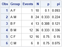
This pilot study has 107 subjects. The first group ("A F") contained 10 subjects, which is π1 = 9.3% of the total. In the first group, one person experienced the event, which is p1 = 10% of the group. The other rows of the table are similar. Some people call this "event-trials" data because the quantity of interest is the proportion of events that occurred in the subjects. The next section shows how to use these estimates to simulate new data samples.
Simulate group sizes and proportions in groups
One of the advantages of simulation studies is that you can take preliminary data from a pilot study and "scale it up" to create larger samples, assuming that the statistics from the pilot study are representative of the parameters in the population. For example, the pilot study involved 107 subjects, but you can easily simulate samples of size 250 or 1000 or more.
The following SAS/IML program simulates samples of size 250. The statistics from the pilot study are used as parameters in the simulation. For example, the simulation assumes that 0.093 of the population belongs to the first group, and that 10% of the subjects in the first group experience the event of interest. Notice that some groups will have a small number of subjects (such as Group 1 and Group 5, which have small values for π). Among the groups, some will have a small proportion of events (Group 1) whereas others will have a large proportion (Group 5 and Group 6).
The following simulation uses the following features:
- The RandMultinomial function in SAS/IML generates a random set of samples sizes based on the π vector, which estimates the proportion of the population that belongs to each group.
- For each group, you can use the binomial distribution to randomly generate the number of events in the group.
- The proportion of events is the ratio (Number of Events) / (Group Size).
/* simulate proportions of events in groups */ proc iml; use Events; read all var _ALL_; /* creates vectors Groups, Events, N, p, pi, etc */ close; numGroups = nrow(Group); call randseed(12345); nTrials = 250; /* simulate data for a study that contains 250 subjects */ Size = T( RandMultinomial(1, nTrials, pi) ); /* new random group sizes */ nEvents = j(numGroups, 1, .); /* vector for number of events */ do i = 1 to nrow(nEvents); nEvents[i] = randfun(1, "Binomial", p[i], Size[i]); end; Proportion = nEvents / Size; /* proportion of events in each group */ results = Size || nEvents || Proportion; print results[r=Group c={'Size' 'nEvents' 'Proportion'} F=Best5.]; |
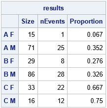
The table shows one random sample of size 250 based on the statistics in the smaller pilot study. The group size and the number of events are both random variables. If you rerun this simulation, the number of subjects in the groups will change, as will the proportion of subjects in each group that experience the event. It would be trivial to adapt the program to handle a designed experiment in which the Size vector is constant.
Simulating multiple samples
An important property of a Monte Carlo simulation study is that it reveals the distribution of statistics that can possibly result in a future data sample. The table in the previous section shows one possible set of statistics, but we can run the simulation additional times to generate hundreds or thousands of additional variations. The following program generates 1,000 possible random samples and outputs the results to a SAS data set. You can then graph the distribution of the statistics. This section uses box plots to visualize the distribution of the proportion of events in each group:
/* simulate 1000 random draws under this model */ SampleID = j(numGroups, 1, .); nEvents = j(numGroups, 1, .); /* vector for number of events */ create Sim var {'SampleID' 'Group' 'Size' 'nEvents' 'Proportion'}; do ID = 1 to 1000; /* assign all elements the same value: https://blogs.sas.com/content/iml/2013/02/18/empty-subscript.html */ SampleID[,] = ID; Size = T( RandMultinomial(1, nTrials, pi) ); /* new random group sizes */ do i = 1 to nrow(nEvents); nEvents[i] = randfun(1, "Binomial", p[i], Size[i]); end; Proportion = nEvents / Size; append; end; close Sim; QUIT; data PlotAll; set Sim Events(keep=Group p); run; title "Proportion of Events in Each Group"; title2 "Simulated N=250; NumSim=1000"; /* box plot */ proc sgplot data=PlotAll noautolegend; hbox Proportion / category=Group; scatter y=Group x=p / markerattrs=GraphData2(symbol=CircleFilled size=11); yaxis type=discrete display=(nolabel); /* create categorical axis */ xaxis grid; run; |
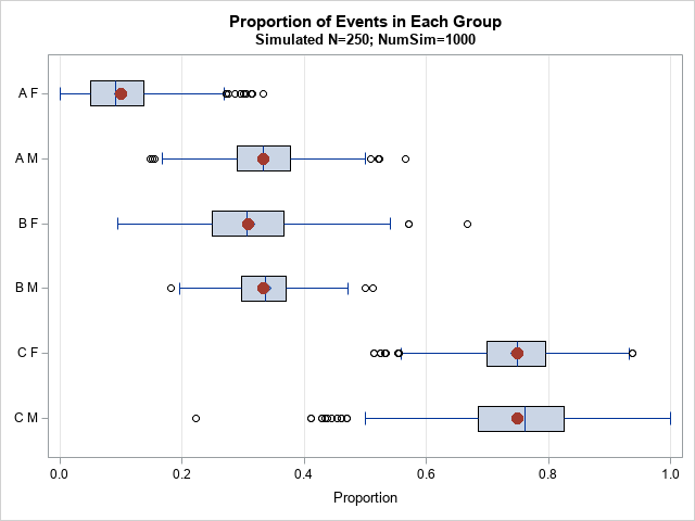
The box plot shows the distribution of the proportion of events in each group. For example, the proportion in the first group ("A F"), ranges from a low of 0% to a high of 33%. The proportion in the sixth group ("C M"), ranges from a low of 22% to a high of 100%. The red markers are the parameter values used in the simulation. These are the estimates from the pilot study.
Alternative ways to visualize the distribution within groups
The box plot shows a schematic representation of the distribution of proportions within each group. However, there are alternative ways to visualize the distributions. One way is to use a strip plot, as follows:
/* strip plot */ proc sgplot data=PlotAll noautolegend; scatter y=Group x=Proportion / jitter transparency=0.85 /* handle overplotting */ markerattrs=(symbol=CircleFilled); scatter y=Group x=p / markerattrs=(symbol=CircleFilled size=11); yaxis type=discrete reverse display=(nolabel); /* create categorical axis */ xaxis grid; run; |
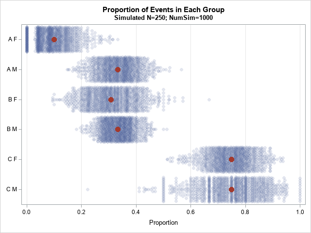
The strip plot uses a semi-transparent marker to display each statistic. (Again, the red markers indicate the parameters for the simulation.) The density of the distribution is visualized by the width of the strips and by the darkness of the plot, which is due to overplotting the semi-transparent markers.
This plot makes it apparent that the variation between groups is based on the relative size of the groups in the pilot study. Large groups such as Group 4 ("B M") have less variation than small groups such as Group 6 ("C M"). That's because the standard error of the proportion is inversely proportional to the square root of the sample size. Thus, smaller groups have a wider distribution than the larger groups.
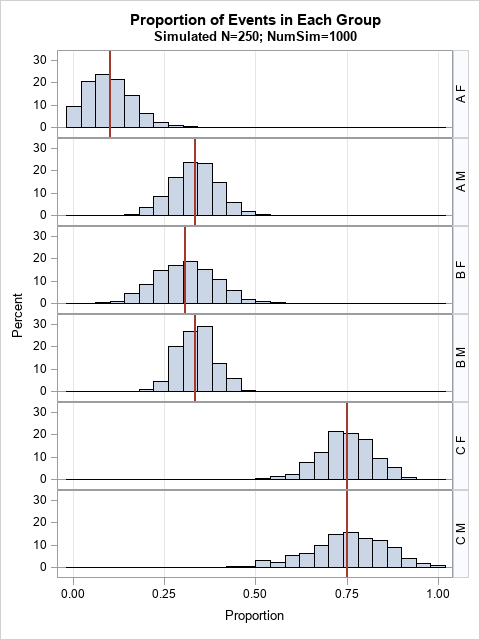
You can see the same features in a panel of histograms. In the following visualization, the distribution of the proportions is shown by using a histogram. Red vertical lines indicate the parameters for the simulation. This graph might be easier to explain to non-statistician./* plot of histograms */ proc sgpanel data=PlotAll; panelby Group / onepanel layout=rowlattice novarname; histogram Proportion; refline p / axis=x lineattrs=GraphData2(thickness=2); colaxis grid; run; |
Summary
This article shows how to simulate event-trials data in SAS. In this example, the data belong to six different groups, and the probability of experiencing the event varies between groups. The groups are also different sizes. In the simulation, the group size and the number of events in each group are random variables. This article also shows three different ways to visualize the results of the simulation: a box plot, a strip plot, and a panel of histograms.
