The SAS DATA step supports multidimensional arrays. However, matrices in SAS/IML are like mathematical matrices: they are always two dimensional. In simulation studies you might need to generate and store thousands of matrices for a later statistical analysis of their properties. How can you accomplish that unless you can create an array of matrices?

A simple solution is to "flatten" each matrix into a row vector and form a big array where the ith row of the array contains the elements of the ith matrix. This storage scheme will be familiar to programmers who have used SAS/IML functions for generating random matrices, such as the RANDWISHART function or my program for generating random symmetric matrices.

Matrices packed into an array

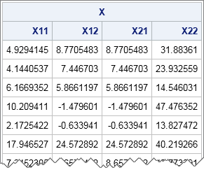
For example, the following example generates 10 random 2 x 2 matrices from a Wishart distribution with 7 degrees of freedom.

proc iml;
call randseed(1234);
DF = 7;
S = {1 1, 1 5};
X = RandWishart(1000, DF, S);   /* generate 1,000 2x2 matrices */
print (X[1:10,])[label="X" colname={X11 X12 X21 X22}];

Each row of the X matrix contains the elements of a 2 x 2 matrix in row-major order. That is, the first element each the row is the (1,1)th element of the matrix, the second is the (1,2)th element, the third is the (2,1)th element, and the fourth is the (2,2)th element.

Extracting matrices from an array

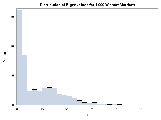
You can use the subscript operator to extract a row from the X array. For example, X[1,] contains the values of the first 2 x 2 matrix. You can use the SHAPE function to reshape each row. This might be necessary if you want to multiply with the matrices or compute their determinant or eigenvalues. For example, the following loop iterates over the rows of the array and computes the eigenvalues of each 2 x 2 matrix. You can use the HISTOGRAM subroutine to plot the distribution of the eigenvalues:

/* compute and store eigenvalues of the 2x2 matrices */
v = j(nrow(X), sqrt(ncol(X)), .);  /* each pxp matrix has p eigenvalues */
do i = 1 to nrow(X);
   A = shape(X[i,], 2);            /* A is symmetric 2x2 matrix */
   v[i,] = T(eigval(A));           /* find eigenvalues; transpose to row vector */
end;
 
title "Distribution of Eigenvalues for 1,000 Wishart Matrices";
call histogram(v) rebin={2.5,5};

The histogram shows a mixture of two distributions. The larger eigenvalue has a mean of 37. The smaller eigenvalue has a mean of 4.5.

Packing matrices into an array

If you have many matrices that are all the same dimension, then it is easy to pack them into an array. Often your program will have a loop that creates the matrices. Within that same loop you can flatten the matrices and pack them into an array. In the following statements, the ROWVEC function is used to convert a square covariance matrix into a row vector.

Z = j(1000, 4, .);                  /* allocate array for 1,000 2x2 matrices */
do i = 1 to nrow(Z);
   Y = randnormal(8, {0 0}, S);     /* simulate 8 obs from MVN(0,S) */
   A = cov(Y);                      /* A is 2x2 covariance matrix */
   Z[i,] = rowvec(A);               /* flatten and store A in i_th row */
end;

The examples in this article have shown how to create a one-dimensional array of matrices. The trick is to flatten the ith matrix and store it in the ith row of a large array. In a similar way, you can build two- or three-dimensional arrays of matrices. Keeping track of which row corresponds to which matrix can be tricky, but the NDX2SUB and SUB2NDX functions can help.

For an alternative technique for working with multidimensional arrays in SAS/IML, see the excellent paper by Michael Friendly, "Multidimensional arrays in SAS/IML Software."