In a previous blog post, I showed how to overlay a prediction ellipse on a scatter plot in SAS by using the ELLIPSE statement in PROC SGPLOT. The ELLIPSE statement draws the ellipse by using a standard technique that assumes the sample is bivariate normal. Today's article describes the technique and shows how to use SAS/IML to compute a prediction ellipse from a 2 x 2 covariance matrix and a mean vector. This can be useful for plotting ellipses for subgroups, ellipses that correspond to robust covariance estimates, or an ellipse for a population (rather than for a sample).
SAS/IML routines for computing prediction ellipses have been around for a long time. A module called the CONTOUR module was in the version 6 (1989) documentation for SAS/IML. In version 6.12, the module was used to compare prediction ellipses for robust and classical covariance matrices. A module appears in Michael Friendly's 1991 book The SAS System for Statistical Graphics, and in several of his papers, including a 1990 SUGI article. Friendly continues to distribute the %ELLIPSES macro for displaying ellipses on scatter plots. The SAS/IML function in this article is similar to these earlier modules.
Prediction ellipses: The main ideas
You can compute a prediction ellipse for sample data if you provide the following information:
- m: A vector for the center of the ellipse.
- S: A covariance matrix. This can be a classical covariance matrix or a robust covariance matrix.
- n: The number of nonmissing observations in the sample.
- p: The confidence level for the prediction ellipse. Equivalently, you could specify a significance level, α, which corresponds to a 1 – α confidence level.
The implicit formula for the prediction ellipse is given in the documentation for the CORR procedure as the set of points that satisfy a quadratic equation.
However, to draw the ellipse, you should parameterize the ellipse explicitly.
For example, when the axes of the ellipse are aligned with the coordinate axes, the equation of an ellipse with center (c,d) and with radii a and b is defined implicitly as the set of points (x,y) that satisfies the equation
(x-c)2 / a2 + (y-d)2 / b2 = 1.
However, if you want to draw the ellipse, the parametric form is more useful:
x(t) = c + a cos(t)
y(t) = d + b sin(t)
for t in the interval [0, 2π].
An algorithm to draw a prediction ellipse
I can think of two ways to draw prediction ellipses. One way is to use the geometry of Mahalanobis distance. The second way, which is used by the classical SAS/IML functions, is to use ideas from principal components analysis to plot the ellipse based on the eigendecomposition of the covariance matrix:
- Find the eigenvalues (λ1 and λ2) and eigenvectors (e1 and e2) of the covariance matrix, S. The eigenvectors form an orthogonal basis for the coordinate system for plotting the ellipse. The first eigenvector (e1) points in the direction of the greatest variance and defines the major axis for the prediction ellipse. The second eigenvector (e2) points in the direction of the minor axis.
-
As mentioned previously, sines and cosines parameterize an ellipse whose axes are aligned with the standard coordinate directions. It is just as simple to parameterize an ellipse in the coordinates defined by the eigenvectors:
- The eigenvectors have unit length, so a circle is formed by the linear combination cos(t)*e1 + sin(t)*e2 for t in the interval [0, 2π].
- The ellipse sqrt(λ1)cos(t)*e1 + sqrt(λ2)sin(t)*e2 is a "standardized ellipse" in the sense that the standard deviations of the variables are used to scale the semi-major axes.
- To get a prediction ellipse, scale the standardized ellipse by a factor that depends on quantiles of the F2,n-2 distribution, the confidence level, and an adjustment factor that depends on the sample size n. The SAS/IML module contains the details.
- Translate the prediction ellipse by adding the vector m.
A SAS/IML module for computing a prediction ellipse
The following module accepts a vector of k confidence levels. The module returns a matrix with three columns. The meaning of each column is described in the comments.
proc iml;
start PredEllipseFromCov(m, S, n, ConfLevel=0.95, nPts=128);
/* Compute prediction ellipses centered at m from the 2x2 covariance matrix S.
   The return matrix is a matrix with three columns.
   Col 1: The X coordinate of the ellipse for the confidence level.
   Col 2: The Y coordinate of the ellipse for the confidence level.
   Col 3: The confidence level. Use this column to extract a single ellipse.

   Input parameters:
   m           a 1x2 vector that specifies the center of the ellipse.
               This can be the sample mean or median.
   S           a 2x2 symmetric positive definite matrix. This can be the
               sample covariance matrix or a robust estimate of the covariance.
   n           The number of nonmissing observations in the data.
   ConfLevel   a 1 x k vector of (1-alpha) confidence levels that determine the
               ellipses. Each entry is 0 < ConfLevel[i] < 1.  For example,
               0.95 produces the 95% confidence ellipse for alpha=0.05.
   nPts       the number of points used to draw the ellipse. The default is 128.
*/

   /* parameterize standard ellipse in coords of eigenvectors */
   call eigen(lambda, evec, S);   /* eigenvectors are columns of evec */
   t = 2*constant("Pi") * (0:nPts-1) / nPts;
   xy  = sqrt(lambda[1])*cos(t) // sqrt(lambda[2])*sin(t);
   stdEllipse = T( evec * xy );   /* transpose for convenience */

   /* scale the ellipse; see documentation for PROC CORR */
   c = 2 * (n-1)/n * (n+1)/(n-2);          /* adjust for finite sample size */
   p = rowvec(ConfLevel);                  /* row vector of confidence levels */
   F = sqrt(c * quantile("F", p, 2, n-2)); /* p = 1-alpha */

   ellipse = j(ncol(p)*nPts, 3);  /* 3 cols: x y p */
   startIdx = 1;                  /* starting index for next ellipse */
   do i = 1 to ncol(p);           /* scale and translate */
      idx = startIdx:startIdx+nPts-1;
      ellipse[idx, 1:2] = F[i] # stdEllipse + m;
      ellipse[idx, 3] = p[i];     /* use confidence level as ID */
      startIdx = startIdx + nPts;
   end;
   return( ellipse );
finish; |
Compare a classical and robust prediction ellipse
The SAS/IML documentation includes an example in which a classical prediction ellipse is compared with a robust prediction ellipse for three-dimensional data that contain outliers. The following SAS/IML statements define the classical and robust estimates of location and scatter for two of the variables. The PredEllipseFromCov function is called twice: once for the classical estimates, which are based on all 21 observations, and once for the robust estimates, which are based on 17 observations:
/* Stackloss data example from SAS/IML doc */
/* classical mean and covariance for stackloss data */
/*      Rate      AcidConcentration */
N = 21;
mean = {60.428571 86.285714};
cov  = {84.057143 24.571429,
        24.571429 28.714286};
classicalEllipse = PredEllipseFromCov(mean, cov, N, 0.9);

/* robust estimates of location and scatter for stackloss data */
/*         Rate      AcidConcentration */
N = 17;
robMean = {56.7      85.5};
robCov  = {23.5     16.1,
           16.1      32.4};
robEllipse = PredEllipseFromCov(robMean, robCov, N, 0.9);

/* write the ellipse data to a SAS data set */
E = classicalEllipse || robEllipse[,1:2];
create Ellipse from E[c={"classX" "classY" "ConfLevel" "robX" "robY"}];
append from E;
close Ellipse;
quit; |
The following SAS statements merge the data and the coordinates for the prediction ellipses. The POLYGON statement in the SGPLOT procedure is used to overlay the ellipses on a scatter plot of the data. The POLYGON statement is available in SAS 9.4M1. Notice that the PredEllipseFromCov function returns a matrix with three columns. The third column (the confidence level) is used as the ID= variable for the POLYGON statement:
data Stackloss; input Rate Temperature AcidCon @@; datalines; 80 27 89 80 27 88 75 25 90 62 24 87 62 22 87 62 23 87 62 24 93 62 24 93 58 23 87 58 18 80 58 18 89 58 17 88 58 18 82 58 19 93 50 18 89 50 18 86 50 19 72 50 19 79 50 20 80 56 20 82 70 20 91 ; data All; set Stackloss Ellipse; run; title "Classical and Robust Prediction Ellipses"; proc sgplot data=All; scatter x=Rate y=AcidCon / transparency=0.5 markerattrs=(symbol=CircleFilled size=12); polygon x=classX y=classY id=ConfLevel / lineattrs=GraphData1 name="classical" legendlabel="Classical 90% Ellipse"; polygon x=robX y=robY id=ConfLevel / lineattrs=GraphData2 name="robust" legendlabel="Robust 90% Ellipse"; xaxis grid; yaxis grid; keylegend "classical" "robust"; run; |
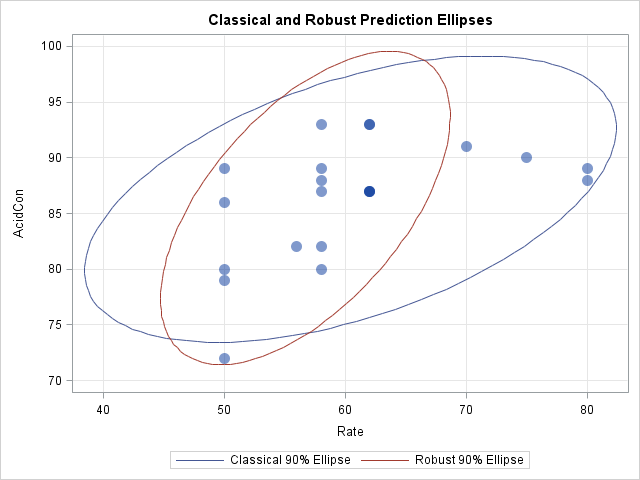
The classical prediction ellipse is based on all 21 observations. The robust estimation method classified four observations as outliers, so the robust ellipse is based on 17 observations. The four outliers are the markers that are outside of the robust ellipse.
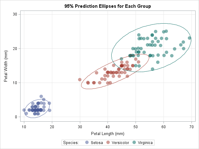
Plotting prediction ellipses for subgroups
You can also use this module to overlay prediction ellipses for subgroups of the data. For example, you can compute the mean and covariance matrix for each of the three species of flower in the sashelp.iris data. You can download the complete program that computes the prediction ellipses and overlays them on a scatter plot of the data. The following graph shows the result:
In summary, by using the SAS/IML language, you can write a short function that computes prediction ellipses from four quantities: a center, a covariance matrix, the sample size, and the confidence level. You can use the function to compute prediction ellipses for classical estimates, robust estimates, and subgroups of the data. You can use the POLYGON statement in PROC SGPLOT to overlay these ellipses on a scatter plot of the data.

8 Comments
Hi Rick,
This series of your remarks on the prediction ellipses are very interesting and entertaining. One request: Could you put up SAS code for what Proc IML does as you had done in some of your blogs? I don't have IML in my SAS installation. Perhaps, Friendly's macro, %ellipses could substitute to generate contents of your SAS data set, ellipse.
Akira
IML is part of SAS. Friendly's macro uses IML, so I assume you are asking for "Base SAS" code that computes the ellipses. I've already shown how to display ellipses with PROC SGPLOT, which is in Base SAS. If you mean that you want the computation done with the DATA step, I'll leave that as "an exercise for the motivated reader." :-)
IMHO, the computation is greatly simplified by using a matrix language. If you want to learn to program in SAS/IML and run the SAS/IML programs in my blog posts, you can download the free SAS University Edition for your personal education and training. As you become proficient in IML, perhaps you can demonstrate to your management how useful it would be to have SAS/IML at your workplace.
Thank you for your reply. I wanted to avoid being a motivated reader but ...
Pingback: Add a prediction ellipse to a scatter plot in SAS - The DO Loop
Pingback: Compute highest density regions in SAS - The DO Loop
Pingback: Generate random uniform points on an ellipse - The DO Loop
Rick,
nPts the number of points used to draw the ellipse. The default is 0.95.
should be
nPts the number of points used to draw the ellipse. The default is 128.
?
Correct.