It is common in statistical graphics to overlay a prediction ellipse on a scatter plot. This article describes two easy ways to overlay prediction ellipses on a scatter plot by using SAS software. It also describes how to overlay multiple prediction ellipses for subpopulations.

What is a prediction ellipse?

A prediction ellipse is a region for predicting the location of a new observation under the assumption that the population is bivariate normal. For example, an 80% prediction ellipse indicates a region that would contain about 80% of a new sample that is drawn from a bivariate normal population with mean and covariance matrices that are equal to the sample estimates.

A prediction ellipse is helpful for detecting deviation from normality. If you overlay a prediction ellipse on your sample and the sample does not "fill" the ellipse in the way that bivariate normal data would, then you have a graphical indication that the data are not bivariate normal.

Because the center of the ellipse is the sample mean, a prediction ellipse can give a visual indication of skewness and outliers in the data. A prediction ellipse also displays linear correlation: If you standardize both variables, a skinny ellipse indicates highly correlated variables, whereas an ellipse that is nearly circular indicates little correlation.

How to draw a prediction ellipse in SAS

SAS provides two easy ways to overlay a prediction ellipse on a scatter plot. The SGPLOT procedure supports the SCATTER statement, which creates a scatter plot, and the ELLIPSE statement, which overlays a bivariate normal prediction ellipse, computed by using the sample mean and covariance. The following statements overlay a 95% prediction ellipse on 50 measurements of the width and length of petals for a particular species of flower:

title "95% Prediction Ellipse";
title2 "iris Versicolor";
proc sgplot data=sashelp.iris noautolegend;
   where Species='Versicolor';
   scatter x=PetalLength y=PetalWidth / jitter;  /* JITTER is optional    */
   ellipse x=PetalLength y=PetalWidth;           /* default is ALPHA=0.05 */
run;

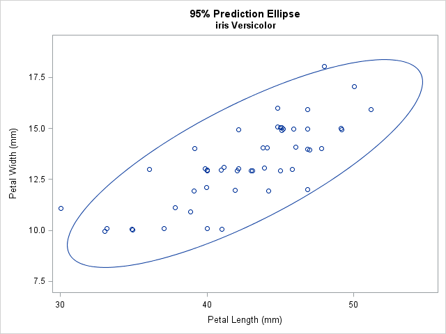
The JITTER option (which requires SAS 9.4) is used to slightly displace some of the observations. Without the option, some markers overlap because the data are rounded to the nearest millimeter. By default, the ELLIPSE statement computes and displays a 95% prediction ellipse, which tends to surround most of the data. However, you can use the ALPHA= option to display a 100(1-α)% prediction ellipse. Some researchers recommend overlaying a 68% prediction ellipse (ALPHA=0.32) because 68% is the probability of observing univariate normal data that is within one standard deviation of the mean. See the article by Michael Friendly for examples and a discussion.

Because a prediction ellipse gives a graphical indication of the linear correlation between variables, you can create a prediction ellipse as part of a correlation analysis in SAS. The following call to the CORR procedure uses the PLOTS=SCATTER option to overlay a 95% prediction ellipse. The output (not shown) is similar to the previous graph.

proc corr data=sashelp.iris plots=scatter(ellipse=prediction);
   where Species='Versicolor';
   var PetalLength PetalWidth;
run;

Draw prediction ellipses for each group

Occasionally, you might want to overlay prediction ellipses for subsets of the data that correspond to subpopulations. For example, if your data contain both male and female subjects, it might be that the means and covariance for the variables are different between males and females. In that case, overlaying a prediction ellipse for each subpopulation helps you to visualize how characteristics vary between the groups.

There are several ways to draw prediction ellipses for groups within the data. Michael Friendly provides a macro that uses SAS/GRAPH to overlay ellipses. It supports a grouping variable, as shown in his 2006 paper in J. Stat. Soft. (This macro has been used in some examples by Robert Allison.)

Edit: Great news! The GROUP= option is supported for the ELLIPSE statement in PROC SGPLOT as of SAS 9.4M3. You not longer need to use the following trick. I will leave it for people who are running older versions of SAS.

If you want to use ODS statistical graphics to display the multiple ellipses, you need to use a little trick. Because the ELLIPSE statement in PROC SGPLOT does not support a GROUP= option as of SAS 9.4m2, you have to reshape the data so that each group becomes a new variable. This is equivalent to transposing the data from a "long form" to a "wide form." From my previous blog post, here is one way to create six variables that represent the petal length and width variables for each of the three species of iris in the sashelp.iris data set:

data Wide;
/*   |-- PetalLength --| |--- PetalWidth ---|  */
keep L_Set L_Vers L_Virg W_Set W_Vers W_Virg;  /* names of new variables */
merge sashelp.iris(where=(Species="Setosa") 
              rename=(PetalLength=L_Set PetalWidth=W_Set))
      sashelp.iris(where=(Species="Versicolor") 
              rename=(PetalLength=L_Vers PetalWidth=W_Vers))
      sashelp.iris(where=(Species="Virginica") 
              rename=(PetalLength=L_Virg PetalWidth=W_Virg));
run;

Now that the data are in separate variables, call PROC SGPLOT to overlay three scatter plots and three 95% prediction ellipses:

title "95% Prediction Ellipses for Each Group";
proc sgplot data=Wide;
  scatter x=L_Set  y=W_Set  / jitter name="Set"  legendlabel="Setosa";
  scatter x=L_Virg y=W_Virg / jitter name="Virg" legendlabel="Virginica";
  scatter x=L_Vers y=W_Vers / jitter name="Vers" legendlabel="Versicolor";
  ellipse x=L_Set  y=W_Set  / lineattrs=GraphData1;
  ellipse x=L_Virg y=W_Virg / lineattrs=GraphData2;
  ellipse x=L_Vers y=W_Vers / lineattrs=GraphData3;
  keylegend "Set" "Virg" "Vers" / title="Species:";
  xaxis label="Petal Length (mm)";
  yaxis label="Petal Width (mm)";
run;

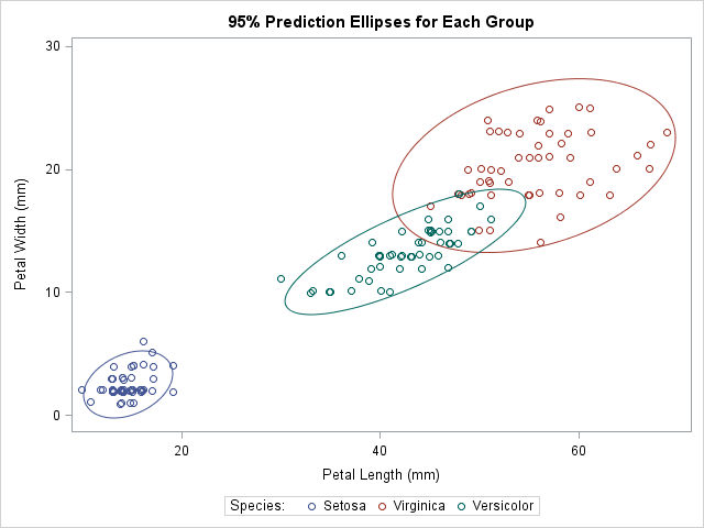
Notice that I used a trick to make the color of each prediction ellipse match the color of the data to which it is associated. The colors for markers in the scatter plots are assigned automatically according to the current ODS style. The style elements used for the markers are named GraphData1, GraphData2, and GraphData3. When I create the ellipses, I use the LINEATTRS= statement to set the style attributes of the ellipse to match the corresponding attributes of the data.

The graph visualizes the relationship between the petal length and the petal width variables in these three species. At a glance, three facts are evident:

• The means of the variables (the centers of the ellipses) are different across the groups. This is a "graphical MANOVA test."
• The Versicolor ellipse is "thinner" than the others, which indicates that the correlation between petal length and width is greater in that species.
• The Virginica ellipse is larger than the others, which indicates greater variance within that species.

In summary, it is easy to use the ELLIPSE statement in PROC SGPLOT to add a prediction ellipse to a scatter plot. If you want to add an ellipse for subgroups of the data, use the trick from my previous article to reshape the data. Plotting ellipses for subgroups enables you to visually inspect covariance and correlation within groups and to compare those quantities across groups. In my next blog post, I will show how to create and plot prediction ellipses directly from a covariance matrix.