I have previously written about how to efficiently generate points uniformly at random inside a sphere (often called a ball by mathematicians). The method uses a mathematical fact from multivariate statistics: If X is drawn from the uncorrelated multivariate normal distribution in dimensiond, then S = r*X / ||X|| has the uniform distribution in the unit ball, where r ~ (1/U)(1/d) and U ~ U(0,1). This is true in any dimension; see the previous article for pictures of a uniform sample inside a ball in 3-D.
It is worth mentioning that this procedure can also be used to generate random points uniformly in any ellipse. This article shows the mathematical algorithm and implements it in SAS. Examples are shown in 2-D (an ellipse in the plane) and in 3-D (an ellipsoid). The same process works for hyperellipsoids in high-dimensional Euclidean space.
From spheres to ellipsoids
Intuitively, you can move from spheres to ellipsoids by changing the covariance matrix that you use for the multivariate normal (MVN) distribution. When the covariance matrix is the identity matrix, the equi-probability contours of the density are spheres. However, for a general positive definite covariance matrix, the equi-probability contours of the density are (hyper)ellipsoids. A particularly simple choice for a covariance matrix is a diagonal matrix. For a diagonal matrix, the axes of the density ellipsoids are orthogonal and are aligned with the standard coordinate axes.
There is a simple geometric relationship between the equi-probability contours for an uncorrelated MVN distribution and for a correlated MVN distribution with covariance matrix Σ. Briefly, if you use the Cholesky factorization to decompose Σ = LLT, then the matrix L is a linear transformation that maps the spherical contours of the uncorrelated distribution to corresponding contours of the correlated distribution, as shown by the image to the right.
The geometry (and the computation) is simplest when you use a diagonal covariance matrix. If \(\Sigma = \mbox{diag}(\sigma_1^2, \sigma_2^2, \ldots, \sigma_d^2)\) is a diagonal covariance matrix, then L = diag(σ1, σ2, ..., σd) for σi > 0. The linear transformation, L, maps the unit sphere at the origin to an ellipsoid with axes that are aligned with the standard coordinate axes and whose radii are σ1, σ2, ..., σd.
The uniform distribution is preserved under a linear transformation
Of course, this problem requires more than mapping a ball to an ellipsoid. We want to generate uniform random variates in an ellipsoid. Fortunately, you can prove that the uniform distribution in a region is preserved under a linear transformation. More precisely, suppose that X is a continuous random variable with a uniform distribution on some subset S in d-dimensional Euclidean space, where S has positive measure. Let Y = μ + L*X be any affine transformation of X, where μ is a d-dimensional vector and L is an invertible d x d matrix. Then Y is uniformly distributed on the image of S, which is the set {y = μ + L*x | x ∈ S}.
Notice that the set S must be a set of positive measure. For example, it must be an area in 2-D, a volume in 3-D, and so forth.
This theorem tells you that you can generate random uniform variates in the unit ball (as shown in the previous article) and then linearly transform those variates to obtain uniform variates in an ellipsoid. The transformed variates will be uniformly distributed in the image of the ball, which is an ellipsoid.
A SAS program to generate random uniform variates in an ellipse
You can carry out this process in any matrix-vector language, such as R, MATLAB, or SAS IML. The following SAS IML program defines a function that takes two arguments: the number of points (n) to generate, and a vector of d positive values, which represent the elements of a diagonal covariance matrix. It returns n points in d-dimensional space that are in the ellipse {y = diag(σ1, σ2, ..., σd)*x | x is in the unit ball and σi > 0}.
/* Uniform random points in an ellipsoid in d-dimensional space. The ellipsoid is the image of the unit ball under the transformation x -> L*x where x is in the ball and L = diag(sigma_1, sigma_2, ..., sigma_d), sigma_i > 0. */ proc iml; /* generate n random uniform points in the ellipse L*x, where x is in unit ball and L = diag(s) */ start RandEllipse(n, s); d = ncol(s); mu = j(1, d, 0); X = randnormal(n, mu, I(d)); /* X ~ N(0, I) */ u = randfun(n, "Uniform"); /* U ~ U(0,1) */ r = u##(1/d); /* r proportional to d_th root of U */ Z = r # X / sqrt(X[,##]); /* uniform in disk or ball */ L = diag(s); /* Cholesky root of covariance matrix Sigma=diag(s##2) */ return Z * L`; /* uniform in ellipse/ellipsoid */ finish; call randseed(12345); /* 2-D example with n=200 points in an ellipse in the plane */ n = 1000; sigmas = {4 3}; Y = RandEllipse(n, sigmas); title "1,000 Random Points in Ellipse"; call scatter(Y[,1], Y[,2]) grid={x y} procopt="aspect=0.75" option="transparency=0.5"; |
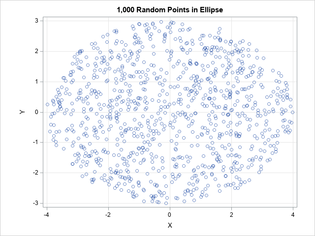
A scatter plot of the output shows that the points are distributed uniformly at random in the ellipse with one axis aligned with the vector (4,0) and the other axis aligned with the vector (0,3).
The same function supports generating points in higher-dimensional ellipsoids. For example, to get random points in an ellipsoid in 3-D, you can use the following statements.
/* 3-D example with points in an ellipsoid */ Y = RandEllipse(5000, {4 3 1}); /* axes aligned with (4,0,0), (0,3,0), and (0,0,1) */ /* write points to a data set and visualize */ create RandEllipsoid from Y[c={'x1' 'x2' 'x3'}]; append from Y; close; QUIT; title "5,000 Random Points in an Ellipsoid"; proc sgplot data=RandEllipsoid; scatter x=x1 y=x2 / colorresponse=x3 transparency=0.5 markerattrs=(symbol=CircleFilled); xaxis grid; yaxis grid; run; |
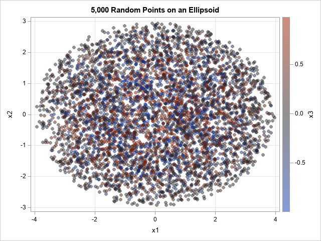
The graph projects the points onto the (x,y) plane. The markers are color-coded according to the z value, which ranges in [-1,1]. Because the points are in an ellipsoid, points that are close to z=0 are located near the planar ellipse that passes through (±4, 0) and (0, ±3). These points are gray in color. Points near the middle of this graph are colored blue, gray, or red, because the z value varies.
Ellipsoids not aligned with the coordinate axis
The same technique works even if you do not use a diagonal covariance matrix. Given any positive definite matrix, you can find the Cholesky decomposition Σ = LLT and use L to map random variate from the unit disk into an ellipse. The following SAS IML function implements this general technique:
proc iml; /* generate n random uniform points in the ellipse L*x, where x is in the unit ball and L satisfies Sigma = L*L` */ start RandEllipseCov(n, Sigma); d = ncol(Sigma); mu = j(1, d, 0); X = randnormal(n, mu, I(d)); /* X ~ N(0, I) */ u = randfun(n, "Uniform"); /* U ~ U(0,1) */ r = u##(1/d); /* r proportional to d_th root of U */ Z = r # X / sqrt( X[,##] ); /* Z is uniform in disk or ball */ U = root(Sigma); /* Cholesky decomp Sigma=U`*U, U upper triangular */ L = U`; /* Sigma=L*L', L lower triangular */ return Z * L`; /* points are uniform in ellipse/ellipsoid */ finish; call randseed(12345); /* 2-D example with n=1,000 points in ellipse in plane */ n = 1000; Sigma = {16 4, 4 9}; Y = RandEllipseCov(n, Sigma); title "1,000 Random Points in a Tilted Ellipse"; /* slopes of reference lines are the directions of the eigenvectors of Sigma */ call scatter(Y[,1], Y[,2]) grid={x y} procopt="aspect=0.75 noautolegend" option="transparency=0.5" other="lineparm x=0 y=0 slope=0.4537682/ lineattrs=(color=gray); lineparm x=0 y=0 slope=-2.203768/lineattrs=(color=gray);"; |
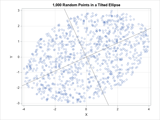
The graph overlays two reference lines, which indicate the axes for the ellipse. They are computed by using the eigenvectors of the Σ matrix. The computation is not shown here, but you can read the details in a previous article about ellipses and covariance matrices.
Summary
This article shows how to generate points uniformly at random in an ellipse, in an ellipsoid, or in any hyperellipsoid in higher dimensions. It first generates points uniformly at random in the unit ball, then uses a linear transformation to map the points into an ellipsoid. If you want an ellipse whose axes are aligned with the coordinate axes, the linear transformation is given by a simple diagonal matrix with positive values on the diagonal. You can also generate points in ellipsoids whose axes are not aligned with the coordinate axes. If Σ is any positive definite matrix, you can decompose Σ = LLT. If you generate points in the unit ball, you can use L to map them into the ellipse whose axes are aligned with the eigendirections of Σ.

6 Comments
Thanks, Rick, for this interesting sequel to your previous article.
I'm not sure I understand your reasoning in section "The uniform distribution is preserved under a linear transformation." The statement in the linked reference (about the uniform distribution being preserved) does not apply to the (d-1)-dimensional sphere S because its d-dimensional volume is zero. Indeed, in the first 2-D example the probability densities near (-4, 0) and (4, 0) are greater than those near (0, 3) and (0, -3), resulting in different expected numbers of random points per unit arc length. Also, in my histograms the marginal distributions of the x- and y-coordinates don't look uniform, but rather U-shaped. (As I don't have a SAS/IML license, I used a data step to reproduce the ellipse dataset. Thanks to the common "MTHybrid" random-number generator I obtained the same 200 points.)
In any random sample from a uniform distribution, there will be gaps and clusters. If you change the random number seed, the gaps and clusters will move to other locations. If you run my first example several times with different seeds, you will see that there is no systematic bias in the distribution of the points.
As to your comment about the marginal histogram, yes, the marginal histogram should be U-shaped. Uniformity on the ellipse does not imply uniformity when the points are projected onto the X or Y axis. In fact, you can prove that if (x,y) is uniformly distributed on the unit circle, that the marginal distribution has the density f(x) = 1/ (pi*sqrt(1-x^2)), which is a U-shaped density on the interval (-1,1).
Thanks for your response. I mentioned the (non-uniform) marginal distributions because you wrote: "You can use histograms to demonstrate that each coordinate has a uniform marginal distribution." Maybe I have misunderstood this sentence.
My first issue is not about the random gaps and clusters of the empirical distribution, but really about the theoretical distribution. It helped me to envision a uniform distribution on a square (rather than a circle), e.g., S={(x, y) in [-1, 1]²: |x|=1 or |y|=1}. Now, if the linear transformation Y = diag(1, 0.5)*X is applied to this square, isn't the probability density on the vertical sides (length=1) of the resulting rectangle twice as large as on the horizontal sides (length=2)? A similar effect should occur when a circle is transformed to an ellipse: The transformation with diag(1, 0.5) -- or even diag(1, 0.001) -- should lead to an increased probability density near the left and right vertices of the resulting ellipse (in comparison to the co-vertices), hence a non-uniform distribution if the distribution on the circle was uniform.
I don't know why I wrote that sentence. It is not correct. Thanks for pointing out my mistake.
Regarding the square and the linear transformation, yes, what you describe is correct. But the term "uniform density" depends on the domain, not just the density function.
For the interval [0,1], the function f(x)=1 is the uniform density function. If I stretch the domain by a factor of 2, then the function g(y)=1/2 is the uniform density on [0,2]. You can read about how to convert one density into another under a linear transformation. For this example, with L=2 being the linear transformation, we have g(y) = (1/L) f(y/L).
I agree that the term "uniform density" depends on the domain. But isn't the characteristic feature of a uniform distribution that the density is constant on its domain (up to null sets)? The distribution in my example is not uniform on the rectangle (where the density takes two different values), so the original uniform distribution on the square was not preserved under the linear transformation. (Which does not contradict the theorem you referred to because it does not apply to null sets such as squares or circles as subsets of the plane.)
The original probability distributions on your circles and spheres are uniform. My point is that the distributions on the ellipses and ellipsoids you obtained by affine transformations are not uniform in the above sense. Their densities vary as you move around those curves/surfaces. As a consequence, when sampling from these distributions, the expected number of random points per unit arc length (surface area or (d-1)-dimensional volume in the general case) varies in the same way. On average, the number of random points in a small neighborhood of one of the vertices of the ellipse (e.g., the image of the circle under the diag(1, 0.5) transformation) will be greater than the corresponding number in a neighborhood of the same size (i.e., arc length) of a point anywhere else on the ellipse.
In what sense are these distributions uniform?
Thank you for your careful reading and patient explanations. Finally, I understand your argument. Yes, you are correct, my original reasoning was flawed. I failed to notice that the linear-transformation theorem applies only to regions of positive measure, such as an area in 2-D, a volume in 3-D, etc. I was trying to apply the theorem to a 1-D circle embedded in 2-D space, and, as you correctly noted, that does not work.
Fortunately, the main idea can be salvaged if we apply the theorem correctly. I rewrote the article to discuss uniform densities inside balls and ellipsoids instead of on the boundary of these regions. You might need to refresh your browser cache (or use Private/Incognito mode) to see the new images, which are now inside ellipses or ellipsoids.