Suppose you roll six identical six-sided dice. Chance are that you will see at least one repeated number. The probability that you will see six unique numbers is very small: only 6! / 6^6 ≈ 0.015.

This example can be generalized. If you draw a random sample with replacement from a set of n items, duplicate values occur much more frequently than most people think. This is the source of the famous "birthday matching problem" in probability, which shows that the probability of duplicate birthdays among a small group of people is higher than most people would guess. (Among 23 people, the probability of a duplicate birthday is more than 50%.)

This fact has implications for bootstrap resampling. Recall that if a sample has n observations, then a bootstrap sample is obtained by sampling n times with replacement from the data. Since most bootstrap samples contain a duplicate of at least one observation, it is also true that most samples omit at least one observation. That raises the question: On average, how many of the original observations are not present in an average bootstrap sample?

The average bootstrap sample

I'll give you the answer: an average bootstrap sample contains 63.2% of the original observations and omits 36.8%. The book by Chernick and LaBudde (2011, p. 199) states the following result about bootstrap resamples: "If the sample size is large and we [generate many]  bootstrap samples, we will find that on average, approximately 36.8% of the original observations will be missing from the individual bootstrap samples. Another way to look at this is that for any particular observation, approximately 36.8% of the bootstrap samples will not contain it." (Emphasis added.)

You can use elementary probability to derive this result. Suppose the original data contains n observations. A bootstrap sample is generated by sampling with replacement from the data. The probability that a particular observation is not chosen from a set of n observations is 1 - 1/n, so the probability that the observation is not chosen n times is (1 - 1/n)^n. This is the probability that the observation does not appear in a bootstrap sample.

You might remember from calculus that the limit as n → ∞ of (1 - 1/n)^n is 1/e. Therefore, when n is large, the probability that an observation is not chosen is approximately 1/e ≈ 0.368.

Simulation: the proportion of observations in bootstrap samples

If you prefer simulation to calculation, you can simulate many bootstrap samples and count the proportion of samples that do not contain observation 1, observation 2, and so forth. The average of those proportions should be close to 1/e.

The theoretical result is only valid for large values of n, but let's start with n=6 so that we can print out intermediate results during the simulation. The following SAS/IML program uses the SAMPLE function to simulate rolling six dice a total of 10 times. Each column of the matrix M contains the result of one trial:

options linesize=128;
proc iml;
call randseed(54321);
n = 6;
NumSamples = 10;
x = T(1:n);                     /* the original sample {1,2,...,n} */
M = sample(x, NumSamples//n);  /* each column is a draw with replacement */

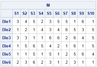
The table shows that each sample (column) contains duplicates. The first column does not contain the values {4,5,6}. The second column does not contain the value 6.

Given these samples, what proportion of samples does not contain 1? What proportion does not contain 2, and so forth? For this small simulation, we can answer these questions by visual inspection. The number 1 does not appear in the sample S5, so it does not appear in 0.1 of the samples. The number 2 does not appears in S3, S5, S8, S9, or S10, so it does not appear in 0.5 of the samples. The following SAS/IML statements count the proportion of columns that do not contain each number and then takes the average of those proportions:

/* how many samples do not contain x[1], x[2], etc */
cnt = j(n, 1, .);     /* allocate space for results */
do i = 1 to n;
   Y = (M=x[i]);      /* binary matrix */
   s = Y[+, ];        /* count for each sample (column) */
   cnt[i] = sum(s=0); /* number of samples that do not contain x[i] */
end;
prop = cnt / NumSamples;
avg_prop = mean(prop);
print avg_prop;

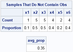
The result says that, on the average, a sample does not contain 0.35 of the data values. Let's increase the sample size and the number of bootstrap samples. Change the parameters to the following and rerun the program:

n = 75;
NumSamples = 10000;

The new estimate is 0.365, which is close to the theoretical value of 1/e. If you like, you can plot a histogram of the n proportions that make up the average:

title "Proportion of Samples That Do Not Contain an Observation";
title2 "n=75; NumSamples=10000";
call histogram(prop) label="Proprtion"
         other="refline "+char(avg_prop)+"/axis=x;";

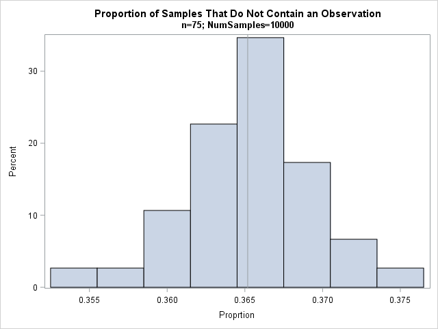
Elementary statistical theory tells us that the proportions are approximately normally distributed with mean p=1/e and standard deviation sqrt(p(1-p)/NumSamples) ≈ 0.00482. The mean and standard deviation of the simulated proportions are very close to the theoretical values.

In conclusion, when you draw n items with replacement from a large sample of size n, on average the sample contains 63.2% of the original observations and omits 36.8%. In other words, the average bootstrap sample omits 36.8% of the original data.