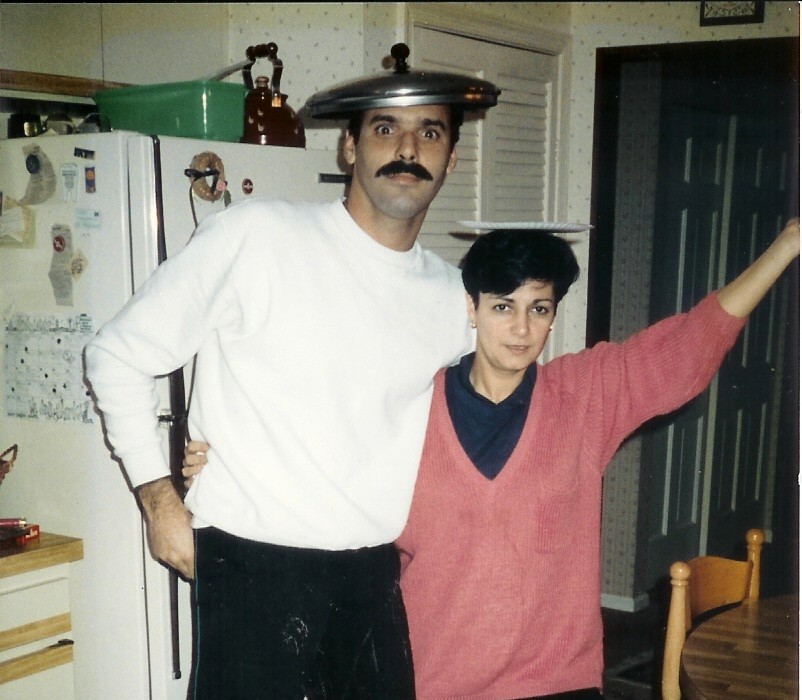
Do you have an Uncle Louie? Yep - we all do! You know what I mean - this guy:
When my wife and I were planning to get married, we had all sorts of big decisions to make. Where would our future home be? How many kids would we have? Joint bank account or individual? Through all of our deliberation, we almost forgot the most important decision of all. Who would have to sit with Uncle Louie at the wedding reception?!
Louie is the standard uncle in a large Italian family. The life of the party - inventor of our great Thanksgiving tradition - The Galati Fart Game (I am not kidding). So, when it came time to assign Uncle Louie to a particular table for the wedding reception, we had a small dilemma. Some family members wanted to be seated with Louie and very much enjoyed his company. Others would probably have rejected the invitation if they had been seated with Louie.
Of course, Uncle Louie is not the only problem:
So... what to do? Luckily, working for SAS and being an optimization guy, I had the idea to build a mathematical model (integer program) to optimize the seat assignments to minimize the overall unhappiness of the guests.
The Optimal Wedding Seat Assignment Problem
A model for this problem was already presented in the paper Dippy – A Simplified Interface for Advanced Mixed-Integer Programming.
Here is the idea. Let's assume that you can collect (or simply know) a measure of unhappiness if guest![g]() were to be seated with guest
were to be seated with guest ![h]() . Let's call this value
. Let's call this value ![a_{gh}]() . The higher the value, the more unhappy guests
. The higher the value, the more unhappy guests ![g]() and
and ![h]() will be with your decision. Let
will be with your decision. Let ![G]() define the set of guests,
define the set of guests, ![T]() define the set of tables available, and
define the set of tables available, and ![S]() define the number of seats available at each table. The unhappiness of a table is defined as the maximum unhappiness of all pairs of guests at a table. The goal is to assign guests to tables so as to minimize the total unhappiness of all the table assignments.
define the number of seats available at each table. The unhappiness of a table is defined as the maximum unhappiness of all pairs of guests at a table. The goal is to assign guests to tables so as to minimize the total unhappiness of all the table assignments.
To model this, let's define a binary decision variable![x_{gt}]() , which will be chosen to be 1 if guest
, which will be chosen to be 1 if guest ![g]() is assigned to table
is assigned to table ![t]() . Let
. Let ![u_t]() define the unhappiness of table
define the unhappiness of table ![t]() . Then, we can formulate the optimization model as the following mixed integer linear programming (MILP) problem:
. Then, we can formulate the optimization model as the following mixed integer linear programming (MILP) problem:
![\begin{align} & \text{minimize} & \sum_{t \in T} u_t \notag \\ & \text{subject to} & \sum_{t \in T} x_{gt} & = 1 & & g \in G \\ & & \sum_{g \in G} x_{gt} & \leq S && t \in T \\ && u_t & \geq a_{gh}(x_{gt} + x_{ht} - 1) && t \in T, g \in G, h \in G \text{ such that } g < h\end{align}]()
Constraint (1) ensures that every guest is assigned to exactly one table. Constraint (2) restricts each table to at most![S]() guests.
Constraint (3) defines
guests.
Constraint (3) defines ![u_t]() , the unhappiness of table
, the unhappiness of table ![t]() , by forcing it to be the maximum
, by forcing it to be the maximum ![a_{gh}]() , for all pairs of guests
, for all pairs of guests ![(g,h)]() that are seated together (i.e., if
that are seated together (i.e., if ![x_{gt} = x_{ht} = 1]() , then
, then ![u_t \geq a_{gh}]() ).
).
PROC OPTMODEL and DECOMP
Using the OPTMODEL procedure in SAS/OR, we can now translate the algebra to code as follows. In order to protect the innocent, we show here the same unhappiness data from the paper (not the real data collected from my family). For the paper, they used the equivalent of random data, by setting![a_{gh} = |g-h|]() .
.
The final result is an assignment of guests to tables (those where ![x_{gt} = 1]() in the optimal solution) and is stored in the data set Assignment.
in the optimal solution) and is stored in the data set Assignment.
Even for a medium-sized wedding, solving this problem with standard MILP techniques (branch-and-cut) can be quite difficult. The inherent symmetry in the model causes most tree-based search methods to spend a good deal of time doing redundant work in order to find an optimal solution. Notice, in this case, that the table identifier is arbitrary. Given a solution, if you move everybody originally at table 1 to table 2 and also move everybody originally at table 2 to table 1, the new solution has the same total unhappiness.
When we solve this problem with our standard MILP solver, it takes quite some time to get a good solution. The progress is shown in the log below (using SAS/OR 13.2). The sum of unhappiness (the objective) is listed in the log under 'BestInteger'. Any feasible solution must have total unhappiness greater than or equal to the 'BestBound'. After 1 hour of computing time, the standard algorithms are still far from finding an optimal solution and proving optimality (as designated under 'Gap').
Now, by simply using the following decomposition option, the wedding assignment problem can be solved much more quickly:
Technical side-note
The automated DECOMP option method=set is a hidden option that detects a set partitioning type of constraint system (as we see in this model). In order to explicitly define the block structures for your model (one subproblem for each table![t]() ), you could use the .block suffix for each constraint. For more details, consult the DECOMP documentation. The syntax to use explicit construction for this model is the following:
), you could use the .block suffix for each constraint. For more details, consult the DECOMP documentation. The syntax to use explicit construction for this model is the following:
In the end, the wedding went off without a hitch. Uncle Louie was relatively tame for most of the night, and we received all positive reviews for the seat assignments. Of course, we forgot to account for this guy...
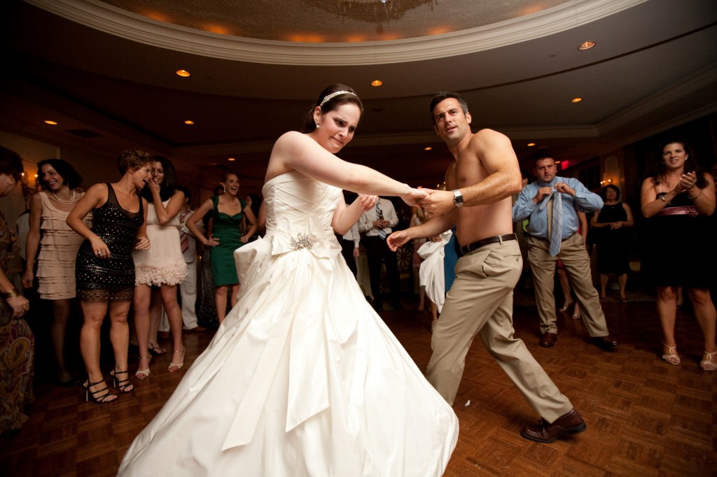 Photo Credit (for the wedding photo): The Wiebners
Disclaimer: The characters in this story are all real. This is not a dramatization.

|
|
Louie is the standard uncle in a large Italian family. The life of the party - inventor of our great Thanksgiving tradition - The Galati Fart Game (I am not kidding). So, when it came time to assign Uncle Louie to a particular table for the wedding reception, we had a small dilemma. Some family members wanted to be seated with Louie and very much enjoyed his company. Others would probably have rejected the invitation if they had been seated with Louie.
Of course, Uncle Louie is not the only problem:
- Aunt Boo had a falling out with Aunt Paula back in the 70s over a leaked muffin recipe and has never forgiven her,
- Tommy Six Toes (second cousin) is a wanted felon in three states while my good friend, James, is a police detective,
- Auntie Sue enjoys throwing her food at people (the adults don't like this, the kids do),
So... what to do? Luckily, working for SAS and being an optimization guy, I had the idea to build a mathematical model (integer program) to optimize the seat assignments to minimize the overall unhappiness of the guests.
The Optimal Wedding Seat Assignment Problem
A model for this problem was already presented in the paper Dippy – A Simplified Interface for Advanced Mixed-Integer Programming.
Here is the idea. Let's assume that you can collect (or simply know) a measure of unhappiness if guest
To model this, let's define a binary decision variable
Constraint (1) ensures that every guest is assigned to exactly one table. Constraint (2) restricts each table to at most
PROC OPTMODEL and DECOMP
Using the OPTMODEL procedure in SAS/OR, we can now translate the algebra to code as follows. In order to protect the innocent, we show here the same unhappiness data from the paper (not the real data collected from my family). For the paper, they used the equivalent of random data, by setting
%macro WeddingPlanner(num_guests=., max_tables=., max_table_size=.); proc optmodel; num num_guests = &num_guests; num max_tables init &max_tables; num max_table_size = &max_table_size; if(max_tables=.) then max_tables = ceil(num_guests / max_table_size); set GUESTS = 1..num_guests; set TABLES = 1..max_tables; set GUEST_PAIRS = {g in 1..num_guests-1, h in g+1..num_guests}; var x{GUESTS,TABLES} binary; var unhappy{TABLES} >= 0; min MinUnhappy = sum{t in TABLES} unhappy[t]; con AssignCon{g in GUESTS}: sum{t in TABLES} x[g,t] = 1; con TableSizeCon{t in TABLES}: sum{g in GUESTS} x[g,t] <= max_table_size; con TableMeasureCon{t in TABLES, <g,h> in GUEST_PAIRS}: unhappy[t] >= abs(g-h) * (x[g,t] + x[h,t] - 1); solve with milp / maxtime=3600; create data Assignment from [guest table]= {g in GUESTS, t in TABLES : x[g,t] > 0.5} x[g,t]; quit; %mend WeddingPlanner; %WeddingPlanner(num_guests=70,max_table_size=6); |
Even for a medium-sized wedding, solving this problem with standard MILP techniques (branch-and-cut) can be quite difficult. The inherent symmetry in the model causes most tree-based search methods to spend a good deal of time doing redundant work in order to find an optimal solution. Notice, in this case, that the table identifier is arbitrary. Given a solution, if you move everybody originally at table 1 to table 2 and also move everybody originally at table 2 to table 1, the new solution has the same total unhappiness.
When we solve this problem with our standard MILP solver, it takes quite some time to get a good solution. The progress is shown in the log below (using SAS/OR 13.2). The sum of unhappiness (the objective) is listed in the log under 'BestInteger'. Any feasible solution must have total unhappiness greater than or equal to the 'BestBound'. After 1 hour of computing time, the standard algorithms are still far from finding an optimal solution and proving optimality (as designated under 'Gap').
NOTE: The presolved problem has 852 variables, 29062 constraints, and 88620
      constraint coefficients.
NOTE: The MILP solver is called.
          Node  Active    Sols    BestInteger      BestBound      Gap    Time
             0       1       0              .              0        .       2
NOTE: The MILP solver's symmetry detection found 36 orbits. The largest orbit
      contains 24 variables.
             0       1       0              .              0        .       3
             0       1       0              .              0        .      10
NOTE: The MILP solver added 25 cuts with 186 cut coefficients at the root.
           100      33       0              .      9.0000000        .      27
           200      65       0              .     10.0000000        .      40
           300      97       0              .     10.4743428        .      52
           400     131       0              .     11.0000000        .      64
           483     162       1    283.0000000     11.0000000 2472.73%      75
           500     171       1    283.0000000     11.0000000 2472.73%      76
           600     204       1    283.0000000     11.1803643 2431.22%      87
-- snip --
         46600   43154      12     94.0000000     12.9549906  625.59%    3573
         46700   43246      12     94.0000000     12.9573416  625.46%    3582
         46800   43338      12     94.0000000     12.9614975  625.22%    3591
         46896   43430      12     94.0000000     12.9618351  625.21%    3599
NOTE: CPU time limit reached.
NOTE: Objective of the best integer solution found = 94.
Fortunately, in the suite of SAS/OR solvers (embedded in PROC OPTMODEL) we also offer the DECOMP algorithm, which provides an alternative approach for solving specially structured MILP problems. In this particular case, DECOMP can automatically detect the symmetry, reformulate the algebraic model into what is known as the Dantzig-Wolfe reformulation, aggregate the symmetric pieces of the model, and use a specialized algorithm under the hood to solve the MILP. For more details on the methodology, consult the Decomposition Algorithm chapter in SAS/OR 13.2 User's Guide: Mathematical Programming (or contact me - the ideas behind this algorithm are the basis of my PhD thesis).
Now, by simply using the following decomposition option, the wedding assignment problem can be solved much more quickly:
solve with milp / decomp=(method=set); |
NOTE: The presolved problem has 852 variables, 29062 constraints, and 88620
      constraint coefficients.
NOTE: The MILP solver is called.
NOTE: The DECOMP method value SET is applied.
NOTE: All blocks are identical and the master model is set partitioning.
NOTE: The Decomposition algorithm is using an aggregate formulation and
      Ryan-Foster branching.
NOTE: The problem has a decomposable structure with 12 blocks. The largest
      block covers 8.31% of the constraints in the problem.
NOTE: The decomposition subproblems cover 852 (100.00%) variables and 28992
      (99.76%) constraints.
NOTE: The deterministic parallel mode is enabled.
NOTE: The Decomposition algorithm is using up to 4 threads.
      Iter         Best       Master         Best       LP       IP  CPU Real
                  Bound    Objective      Integer      Gap      Gap Time Time
NOTE: Starting phase 1.
         1       0.0000      70.0000            . 7.00e+01        .    0    0
        10       0.0000      56.5000            . 5.65e+01        .    0    0
        20       0.0000      44.6000            . 4.46e+01        .    0    0
        30       0.0000      35.8618            . 3.59e+01        .    0    0
        40       0.0000      25.3660            . 2.54e+01        .    0    0
        50       0.0000      16.6091            . 1.66e+01        .    0    0
        60       0.0000       4.3861            . 4.39e+00        .    0    0
        70       0.0000       0.0271            . 2.71e-02        .    0    0
        71       0.0000       0.0000            .    0.00%        .    0    0
NOTE: Starting phase 2.
        76       0.0000     112.0000     112.0000 1.12e+02 1.12e+02    0    0
        80       0.0000     112.0000     112.0000 1.12e+02 1.12e+02    0    1
        90       0.0000     112.0000     112.0000 1.12e+02 1.12e+02    1    1
-- snip --
       460      46.0000      58.0000      58.0000   26.09%   26.09%  157   90
       470      46.0000      58.0000      58.0000   26.09%   26.09%  165   94
       480      50.0000      58.0000      58.0000   16.00%   16.00%  176   99
       483      52.0000      58.0000      58.0000   11.54%   11.54%  178  100
       485      58.0000      58.0000      58.0000    0.00%    0.00%  180  101
         Node  Active   Sols         Best         Best      Gap    CPU   Real
                                  Integer        Bound            Time   Time
            0       0     26      58.0000      58.0000    0.00%    180    101
NOTE: The Decomposition algorithm used 4 threads.
NOTE: The Decomposition algorithm time is 101.69 seconds.
NOTE: Optimal.
NOTE: Objective = 58.
Technical side-note
The automated DECOMP option method=set is a hidden option that detects a set partitioning type of constraint system (as we see in this model). In order to explicitly define the block structures for your model (one subproblem for each table
for{t in TABLES} do; TableSizeCon[t].block = t; for{<g,h> in GUEST_PAIRS} TableMeasureCon[t,g,h].block = t; end; solve with milp / decomp=(method=user); |
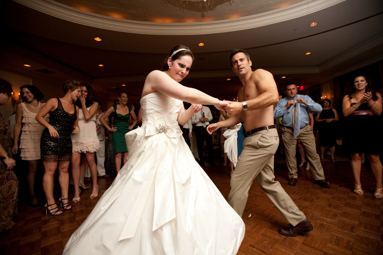 Photo Credit (for the wedding photo): The Wiebners
Disclaimer: The characters in this story are all real. This is not a dramatization.

5 Comments
What about the integer for dudes who taught you how to do a duck under and did not make the cut. I would like to see the data on how this list was developed.
The alternative method would be in-vivo JIT Brownian Motion Optimization, also known as the guests figure it out ;). Humans are really good in clustering and de-clustering based on relationships.
I wonder what the probability of the concerned persons ever even showing up are.
Pingback: The Kidney Exchange Problem - Operations Research with SAS
Pingback: The kidney exchange problem - Operations Research with SAS