The following is an excerpt from Cautionary Tales in Designed Experiments by David Salsburg. This book is available to download for free from SAS Press. The book aims to explain statistical design of experiments (DOE) to readers with minimal mathematical knowledge and skills. In this excerpt, you will learn about the origin of Thomas Bayes’ Theorem, which is the basis for Bayesian analysis.

The Reverend Thomas Bayes (1702–1761) was a dissenting minister of the Anglican Church, which means he did not subscribe to the full body of doctrine espoused by the Church. We know of Bayes in the 21^st century, not because of his doctrinal beliefs, but because of a mathematical discovery, which he thought made no sense whatsoever. To understand Bayes’ Theorem, we need to refer to this question of the meaning of probability.

In the 1930s, the Russian mathematician Andrey Kolomogorov (1904–1987) proved that probability was a measure on a space of “events.” It is a measure, just like area, that can be computed and compared. To prove a theorem about probability, one only needed to draw a rectangle to represent all possible events associated with the problem at hand. Regions of that rectangle represent classes of sub-events.

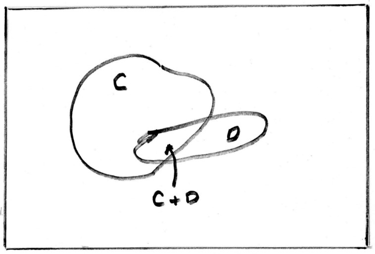
For instance, in Figure 1, the region labeled “C” covers all the ways in which some event, C, can occur. The probability of C is the area of the region C, divided by the area of the entire rectangle. Anticipating Kolomogorov’s proof, John Venn (1834–1923) had produced such diagrams (now called “Venn diagrams”).

Figure 1 shows a Venn diagram for the following situation: We have a quiet wooded area. The event C is that someone will walk through those woods sometime in the next 48 hours. There are many ways in which this can happen. The person might walk in from different entrances and be any of a large number of people living nearby. For this reason, the event C is not a single point, but a region of the set of all possibilities. The event D is that the Toreador Song from the opera Carmen will resound through the woods. Just as with event C, there are a number of ways in which this could happen. It could be whistled or sung aloud by someone walking through the woods, or it could have originated from outside the woods, perhaps from a car radio on a nearby street. Some of these possible events are associated with someone walking through the woods, and those possible events are in the overlap between the regions C and D. Events associated with the sound of the Toreador Song that originate outside the woods are in the part of region D that does not overlap region C.

The area of region C (which we can write P(C) and read it as “P of C”) is the probability that someone will walk through the woods. The area of region D (which we can write P(D)) is the probability that the Toreador Song will be heard in the woods. The area of the overlap between C and D (which we can write P(C and D) is the probability that someone will walk through the woods and that the Toreador Song will be heard.

If we take the area P(C and D) and divide it by the area P(C), we have the probability that the Toreador Song will be heard when someone walks through the woods. This is called the conditional probability of D, given C. In symbols

P(D|C) = P(C and D)÷ P(C)

Some people claim that if the conditional probability, P(C|D), is high, then we can state “D causes C.” But this would get us into the entangled philosophical problem of the meaning of “cause and effect.”

To Thomas Bayes, conditional probability meant just that—cause and effect. The conditioning event, C, (someone will walk through the woods in the next 48 hours) comes before the second event D, (the Toreador Song is heard). This made sense to Bayes. It created a measure of the probability for D when C came before.

However, Bayes’ mathematical intuition saw the symmetry that lay in the formula for conditional probability:

P(D|C) = P(D and C)÷ P(C) means that

P(D|C)P(C) = P(D and C) (multiply both sides of the equation by P(C)).

But just manipulating the symbols shows that, in addition,

P(D and C) = P(C|D) P(D), or

P(C|D) = P(C and D)÷ P(D).

This made no sense to Bayes. The event C (someone walks through the woods) occurred first. It had already happened or not before event D (the Toreador Song is heard). If D is a consequence of C, you cannot have a probability of C, given D. The event that occurred second cannot “cause” the event that came before it. He put these calculations aside and never sent them to the Royal Society. After his death, friends of Bayes discovered these notes and only then were they sent to be read before the Royal Society of London. Thus did Thomas Bayes, the dissenting minister, become famous—not for his finely reasoned dissents from church doctrine, not for his meticulous calculations of minor problems in astronomy, but for his discovery of a formula that he felt was pure nonsense.

P(C|D) P(D) = P(C and D) = P(D|C) P(C)

For the rest of the 18^th century and for much of the 19^th century, Bayes’ Theorem was treated with disdain by mathematicians and scientists. They called it “inverse probability.” If it was used at all, it was as a mathematical trick to get around some difficult problem. But since the 1930s, Bayes’ Theorem has proved to be an important element in the statistician’s bag of “tricks.”

Bayes saw his theorem as implying that an event that comes first “causes” an event that comes after with a certain probability, and an event that comes after “causes” an event that came “before” (foolish idea) with another probability. If you think of Bayes’ Theorem as providing a means of improving on prior knowledge using the data available, then it does make sense.

In experimental design, Bayes’ Theorem has proven very useful when the experimenter has some prior knowledge and wants to incorporate that into his or her design. In general, Bayes’ Theorem allows the experimenter to go beyond the experiment with the concept that experiments are a means of continuing to develop scientific knowledge.

To learn more about how probability is used in experimental design, download Cautionary Tales in Designed Experiments now!