Sort the rows or columns of a matrix independently

When you have a data matrix, the rows represent observations and the columns represent variables. If you sort the matrix by one or more columns, the sorting occurs in a way that preserves the elements within rows. Although the rows of the sorted matrix are permuted by the sort, the sorted matrix is still a data matrix, but now the observations are in a different order.

However, there are instances in which a numerical matrix is merely a way to organize a bunch of numbers. For example, in a simulation study, you might construct a matrix whose i_th column contains the generated data that results from the i_th independent random sample. In this instance, sorting each column of the matrix is useful in analyzing the sampling distribution of the quantiles. For example, if you sort all columns, then the first row of the sorted matrix contains the distribution of the minimum statistic, and the last row contains the distribution of the maximum statistic.

This article shows how to sort the rows and columns of a matrix independently in the SAS IML matrix language.

A matrix from a simulation study

Suppose you want to run a simulation study to approximate the sampling distribution of quantiles in small, normally distributed, random samples. You decide to study samples of size N=25 and you want to graph the approximate distribution of the quantiles based on generating B samples from N(0,1).

In a matrix language like SAS IML, it is efficient to simulate all random samples by using a single call to the RANDFUN functions. You can fill an N x B matrix with N(0,1) variates and interpret each column as a random sample of size N. In a real simulation study, you would choose a large number for B (such as 10,000), but for this article I will choose only B=200 samples because I want to show some visualizations by using a heat map. The following SAS IML program generates the data for the simulation study:

proc iml;
/* simulation study: If X ~ N(0,1), 
   what is the distribution of the sample quantiles? */
N = 25;                      /* sample size */
B = 200;                     /* number of simulations of X ~ N(0,1) */
call randseed(1234);
M = randfun(N//B, "Normal"); /* NxB matrix; each col is random sample */

If you sort each column in the matrix, then it is easier to compute certain rank-based statistics and quantiles. For example, in the sorted matrix, the first row will contain the minimum values for each sample. Similarly, the last row contains the maximum values, and the 13th row contains the median values. (You could also use the QNTL function, which computes quantiles for each column in a matrix.)

Sorting each column of a matrix

If you use CALL SORT in IML (or the SORT procedure in Base SAS), the rows of the matrix are arranged in order according to one or more key columns. To sort the columns independently, you need to loop over the columns, sort each one, and then overwrite the column with the sorted version.

The following IML module, SortCols, sorts the columns of the matrix in either ascending or descending order. You can sort the rows of a matrix by passing in the transpose of the matrix and then transposing the result, as shown in the SortRows function.

/* sort the columns of a matrix independently */
start SortCols(M, descend=0);
  S = M;
  if ^descend then do;
     do i = 1 to ncol(S);
        x = S[,i];
        call sort(x);        /* sort each column in ascending order */
        S[,i] = x;
     end;
  end;
  else do;
     do i = 1 to ncol(S);
        x = S[,i];
        call sort(x, 1, 1); /* sort each column in descending order */
        S[,i] = x;
     end;
  end;
  return( S );
finish;
 
/* sort the rows of a matrix independently. Just call SortCols on the transpose! */
start SortRows(M, descend=0);
  return( T(SortCols(M`, descend)) );
finish;
store module=(SortCols SortRows);
 
/* sort matrix by cols and make a heat map to visualize the result */
t = "Matrix Sorted Ascending by Cols";
A = SortCols(M);
ods graphics / width=480px height=240px;
call heatmapcont(A) colorramp="ThreeColor" displayoutlines=0 xaxistop=1 title=t;
/* Note: To sort the columns in descending order, use 
   A = SortCols(M, 1);
*/

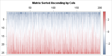
The heat map visualizes the column-wise sorting. For each column, the values in the sorted matrix are stored in increasing order. Thus, the first row contains the smallest value in each sample, the second row contains the second smallest value, and so on, until the last row, which contains the largest value in each sample. Equivalently, each column contains the order statistics for the sample.

If you want to analyze, for example, the distribution of the minimum values in the samples, you can extract the first row. The following statements extract the first row and create a histogram of the sampling distribution of the minimum statistic:

/* The smallest values are in the first row of the sorted matrix */
sample_min = A[1,];
title "Distribution of the Sample Min for N(0,1) Data";
call histogram(sample_min);

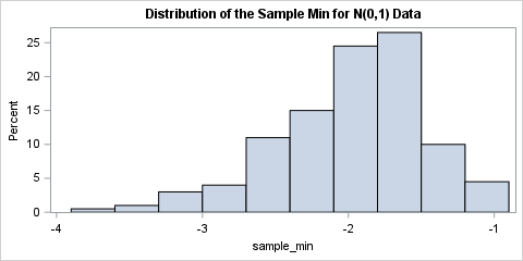
The histogram shows the distribution of the minimum statistic. This distribution is one of the extreme-value distributions, known as the Gumbel distribution. For a standardized normal sample of this size, it is common that the minimum value is near -2, but values less than -3 are possible.

Sorting each row of a matrix

In the same way, you can call the SortRows function to independently sort each row of a matrix:

/* Suppose you organize the simulation so that each row is a random sample. Then the
   simulated samples are the rows of M`. You can sort the rows by calling the SortRows function. */
M = M`;
t = "Matrix Sorted Ascending by Rows";
B = SortRows(M);
ods graphics / width=280px height=480px;
call heatmapcont(B) colorramp="ThreeColor" displayoutlines=0 xaxistop=1 title=t;
/* To sort in descending order, use
B = SortRows(M, 1);  */

Instead of generating new data, I simply transposed the previous simulated matrix. For the transposed matrix, each row is a random sample. If you sort by rows, the columns contain the distributions of the quantiles. The i_th column contains the i_th smallest value in each sample.

Summary

This article shows how to sort each column or each row of a matrix in the SAS IML language. One application is that you can easily analyze the distribution of order statistics, including minima, maxima, and other quantiles. Another application is to sort the columns of a lasagna plot, which can visualize changes to the distribution of a response variable over time.

Blogs