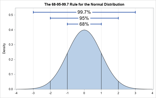
Is 4 an extreme value for the standard normal distribution? In high school, students learn the famous 68-95-99.7 rule, which is a way to remember that 99.7 percent of random observation from a normal distribution are within three standard deviations from the mean. For the standard normal distribution, the probability that a random value is bigger than 3 is 0.0013. The probability that a random value is bigger than 4 is even smaller: about 0.00003 or 3 x 10^-5.

So, if you draw randomly from a standard normal distribution, it must be very rare to see an extreme value greater than 4, right? Well, yes and no. Although it is improbable that any ONE observation is more extreme than 4, if you draw MANY independent observations, the probability that the sample contains an extreme value increases with the sample size. If p is the probability that one observation is less than 4, then pⁿ is the probability that n independent observations are all less than 4. Thus 1 – pⁿ is the probability that some value is greater than 4. You can use the CDF function in SAS to compute these probabilities in a sample of size n:

/* What is a "large value" of a normal sample? The answer depends on the size of the sample. */
/* Use CDF to find probability that a random value from N(0,1) exceeds 4 */
proc iml;
P_NotGT4 = cdf("Normal", 4);   /* P(x < 4) */
 
/* Probability of an extreme obs in a sample that contains n independent observations */
n = {1, 100, 1000, 10000};     /* sample sizes */
P_NotGT4 = P_NotGT4**n;        /* P(all values are < 4) */
P_GT4 = 1 - P_NotGT4;          /* P(any value is > 4)   */
print n P_NotGT4 P_GT4;

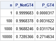
The third column of the table shows that the probability of seeing an observation whose value is greater than 4 increases with the size of the sample. In a sample of size 10,000, the probability is 0.27, which implies that about one out of every four samples of that size will contain a maximum value that exceeds 4.

The distribution of the maximum in a Gaussian sample: A simulation approach

You can use a simulation to approximate the distribution of the maximum value of a normal sample of size n. For definiteness, choose n = 1,000 and sample from a standard normal distribution N(0,1). The following SAS/IML program simulates 5,000 samples of size n and computes the maximum value of each sample. You can then graph the distribution of the maximum values to understand how the maximum value varies in random samples of size n.

/* What is the distribution of the maximum value in a 
   sample of size n drawn from the standard normal distribution? */
call randseed(12345);
n = 1000;                  /* sample size */
numSim = 5000;             /* number of simulations */
x = j(n, numSim);          /* each column will be a sample */
call randgen(x, "Normal"); /* generate numSim samples */
max = x[<>, ];             /* find max of each sample (column) */
 
Title "Distribution of Maximum Value of a Normal Sample";
title2 "n = 1000";
call histogram(max);
 
/* compute some descriptive statistics */
mean = mean(max`);
call qntl(Q, max`, {0.25 0.5 0.75});
print (mean // Q)[rowname={"Mean" "P25" "Median" "P75"}];

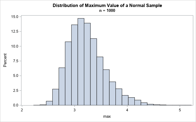
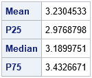
Based on this simulation, the expected maximum value of a sample of size n = 1,000 is about 3.2. The table indicates that about 25% of the samples have a maximum value that is less than 3. About half have a maximum value less than 3.2. About 75% of the samples have a maximum value that is less than 3.4. The graph shows the distribution of maxima in these samples. The maximum value of a sample ranged from 2.3 to 5.2.

The distribution of a maximum (or minimum) value in a sample is studied in an area of statistics that is known as extreme value theory. For large samples, it turns out that you can derive the sampling distribution of the maximum of a sample by using the Gumbel distribution, which is also known as the "extreme value distribution of Type 1." You can use the Gumbel distribution to describe the distribution of the maximum of a sample of size n for large values of n. The Gumbel distribution actually describes the maximum for many distributions, but for simplicity I will only refer to the normal distribution.

The distribution of the maximum in a Gaussian sample: The Gumbel distribution

This section does two things. First, it uses PROC UNIVARIATE to fit the parameters of a Gumbel distribution to the maximum values from the simulated samples. The Gumbel(3.07, 0.29) distribution is the distribution that maximizes the likelihood function for the simulated data. Second, it uses a theoretical formula to show that a Gumbel(3.09, 0.29) distribution is the distribution that models the maximum of a normally distributed sample of size n = 1,000. Thus, the results from the simulation and the theory are similar.

You can write the 5,000 maximum values from the simulation to a SAS data set and use PROC UNIVARIATE to estimate the MLE parameters for the Gumbel distribution, as follows:

create MaxVals var "max"; append; close;
QUIT;
 
/* Fit a Gumbel distribution, which models the distribution of maximum values */
proc univariate data=MaxVals;
   histogram max / gumbel;
   ods select Histogram ParameterEstimates FitQuantiles;
run;

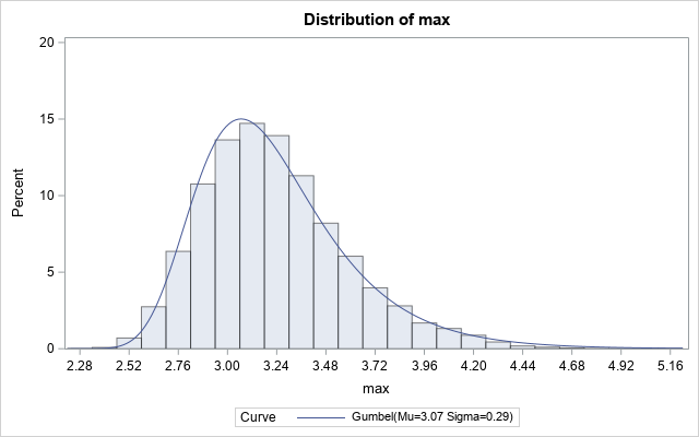
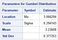
The output from PROC UNIVARIATE shows that the Gumbel(3.07, 0.29) distribution is a good fit to the distribution of the simulated maxima. But where do those parameter values come from? How are the parameters of the Gumbel distribution related to the sample size of the standard normal distribution?

It was difficult to find an online reference that shows how to derive the Gumbel parameters for a normal sample of size n. I finally found a formula in the book Extreme Value Distributions (Kotz and Nadarajah, 2000, p. 9). For any cumulative distribution F that satisfies certain conditions, you can use the quantile function of the distribution to estimate the Gumbel parameters. The result is that the location parameter (μ) is equal to μ = F^-1(1-1/n) and the scale parameter (σ) is equal to σ = F^-1(1-1/(ne)) - μ, where e is the base of the natural logarithm. The following SAS/IML program uses the (1 – 1/n)th quantile of the normal distribution to derive the Gumbel parameters for a normal sample of size n:

proc iml;
n = 1000;
/* Compute parameters of Gumbel distribution when the sample is normal of size n.
   SAS calls the parameters (mu, sigma). Wikipedia calls them (mu, beta). Other
   references use (alpha, beta). */
mu_n    = quantile("Normal", 1-1/n);                /* location parameter */
sigma_n = quantile("Normal", 1-1/n*exp(-1)) - mu_n; /* scale parameter */
print n mu_n sigma_n;
 
/* what is the mean (expected value) and median of this Gumbel distribution? */
gamma = constant("Euler");             /* Euler–Mascheroni constant = 0.5772157 */
mean = mu_n + gamma*sigma_n;           /* expected value of maximum */
median = mu_n - sigma_n * log(log(2)); /* median of maximum value distribution */
print n mean median;

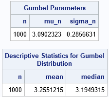
Notice that these parameters are very close to the MLE estimates from the simulated normal samples. The results tell you that the expected maximum in a standard normal sample is 3.26 and about 50% of samples will have a maximum value of 3.19 or less.

You can use these same formulas to find the expected and median values of the maximum in samples of other sizes:

/* If the sample size is n, what is expected maximum */
n = {1E4, 2E4, 1E5, 2E5, 1E6, 2E6};
mu_n    = quantile("Normal", 1-1/n);                /* location parameter */
sigma_n = quantile("Normal", 1-1/n*exp(-1)) - mu_n; /* scale parameter */
mean = mu_n + gamma*sigma_n;           /* expected value of maximum */
median = mu_n - sigma_n * log(log(2)); /* meadian of maximum value distribution */
print n mean median;

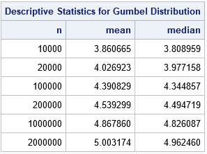
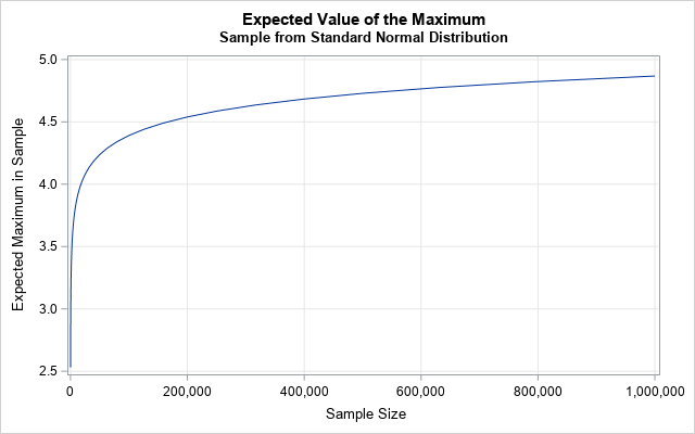
The table shows that you would expect to see a maximum value of 4 in a sample of size 20,000. If there are two million observations in a sample, you would expect to see a maximum value of 5!

You can graph this data over a range of sample sizes. The following graph shows the expected value of the maximum value in a sample of size n (drawn from a standard normal distribution) for large values of n.

You can create similar images for quantiles. The p_th quantile for the Gumbel distribution is q = mu_n - sigma_n log(-log(p)).

So, is 4 an unlikely value for the standard normal distribution? Yes, but for sufficiently large samples that value is likely to be observed. You can use the Gumbel distribution to model the distribution of the maximum in a normal sample of size n to determine how likely it is that the sample contains an extreme value. The larger the sample, the more likely it is to observe an extreme value. Although I do not discuss the general case, the Gumbel distribution can also model the maximum value for samples drawn from some non-normal distributions.